Page 365 - Applied Numerical Methods Using MATLAB

354 OPTIMIZATION

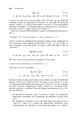
Min f(x) (7.3.4)
s.t. Ax ≤ b,A eq x = b eq , c(x) ≤ 0, c eq (x) = 0 and l ≤ x ≤ u (7.3.5)

A part of its usage can be seen by typing ‘help fmincon’ into the MATLAB
command window as summarized in the above box. We make the MATLAB
program “nm732_1.m”, which uses the routine “fmincon()” to solve the problem
presented in Example 7.3. Interested readers are welcomed to run it and observe
the result to check if it agrees with that of Example 7.3.
There are two more MATLAB built-in routines to be introduced in this section.
One is

"fminimax(’ftn’,x0,A,b,Aeq,beq,l,u,’nlcon’,options,p1,..)",

which is focused on minimizing the maximum among several components of
T
the vector/matrix-valued objective function f(x) = [f 1 (x) ··· f N (x)] subject to
some constraints as described below. Its usage is almost the same as that of
“fmincon()”.

Min{Max{f n (x)}} (7.3.6)
x n
s.t. Ax ≤ b,A eq x = b eq , c(x) ≤ 0, c eq (x) = 0, and l ≤ x ≤ u (7.3.7)

The other is the constrained linear least-squares (LLS) routine

"lsqlin(C,d,A,b,Aeq,beq,l,u,x0,options,p1,..)",

whose job is to solve the problem
2
Min ||Cx − d|| (7.3.8)
x
s.t.Ax ≤ b, A eq x = b eq and l ≤ x ≤ u (7.3.9)

In order to learn the usage and function of this routine, we make the MATLAB
program “nm732_2.m”, whichusesboth“fminimax()”and “lsqlin()”tofind
a second-degree polynomial approximating the function (7.3.3) and compares
the results with that of applying the routine “lsqnonlin()” introduced in the
previous section for verification. From the plotting result depicted in Fig. 7.14,
note the following.

ž We attached no constraints to the “fminimax()” routine, so it yielded the
approximate polynomial curve minimizing the maximum deviation from
f(x).
ž We attached no constraints to the constrained linear least-squares routine
“lsqlin()” either, so it yielded the approximate polynomial curve
minimizing the sum (integral) of squared deviation from f(x),which is