Page 370 - Applied Numerical Methods Using MATLAB

PROBLEMS 359
4

3 5 4 3

2

1

0 6 1 2

−1

−2
8
7 9
−3

−4
−4 −3 −2 −1 0 1 2 3 4
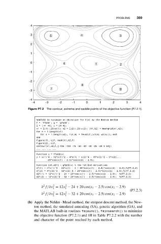
Figure P7.2 The contour, extrema and saddle points of the objective function (P7.2.1).

%nm7p02 to minimize an objective ftn f(x) by the Newton method
f = ’f7p02’; g = ’g7p02’;
l=[-4 -4];u=[44];
x1 = l(1):.25:u(1); x2 = l(2):.25:u(2); [X1,X2] = meshgrid(x1,x2);
for m = 1:length(x1)
for n = 1:length(x2), F(n,m) = feval(f,[x1(m) x2(n)]); end
end
figure(1), clf, mesh(X1,X2,F)
figure(2), clf,
contour(x1,x2,F,[-125 -100 -75 -50 -40 -30 -25 -20 0 50])
... ... ... ...
function y = f7p02(x)
y = x(1)^4 - 12*x(1)^2 - 4*x(1) + x(2)^4 - 16*x(2)^2 - 5*x(2)...
-20*cos(x(1) - 2.5)*cos(x(2) - 2.9);
function [df,d2f] = g7p02(x) % the 1st/2nd derivatives
df(1) = 4*x(1)^3 - 24*x(1)-4+ 20*sin(x(1) - 2.5)*cos(x(2) - 2.9);%(P7.2.2)
df(2) = 4*x(2)^3 - 32*x(2)-5 + 20*cos(x(1) - 2.5)*sin(x(2) - 2.9);%(P7.2.2)
d2f(1) = 12*x(1)^2 - 24 + 20*cos(x(1) - 2.5)*cos(x(2) - 2.9); %(P7.2.3)
d2f(2) = 12*x(2)^2 - 32 + 20*cos(x(1) - 2.5)*cos(x(2) - 2.9); %(P7.2.3)

2
2
2
∂ f/∂x = 12x − 24 + 20 cos(x 1 − 2.5) cos(x 2 − 2.9)
1 1
(P7.2.3)
2
2
2
∂ f/∂x = 12x − 32 + 20 cos(x 1 − 2.5) cos(x 2 − 2.9)
2 1
(b) Apply the Nelder–Mead method, the steepest descent method, the New-
ton method, the simulated annealing (SA), genetic algorithm (GA), and
the MATLAB built-in routines fminunc(), fminsearch() to minimize
the objective function (P7.2.1) and fill in Table P7.2.2 with the number
and character of the point reached by each method.