Page 367 - Applied Numerical Methods Using MATLAB

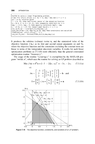
356 OPTIMIZATION

%nm733 to solve a Linear Programming problem.
% Min f*x=-3*x(1)-2*x(2) s.t. Ax <= b, Aeq = beq and l <= x <= u
x0 = [0 0]; %initial point
f = [-3 -2]; %the coefficient vector of the objective function
A = [3 4; 2 1]; b = [7; 3]; %the inequality constraint Ax <= b
Aeq = [-3 2]; beq = 2; %the equality constraint Aeq*x = beq
l = [0 0]; u = [10 10]; %lower/upper bound l <= x <= u
[xo_lp,fo_lp] = linprog(f,A,b,Aeq,beq,l,u)
cons_satisfied = [A; Aeq]*xo_lp-[b; beq] %how constraints are satisfied
f733o=inline(’-3*x(1)-2*x(2)’, ’x’);
[xo_con,fo_con] = fmincon(f733o,x0,A,b,Aeq,beq,l,u)

It produces the solution (column) vector x o and the minimized value of the
objective function f(x o ) as its first and second output arguments xo and fo,
where the objective function and the constraints excluding the constant term are
linear in terms of the independent (decision) variables. It works for such linear
optimization problems as (7.3.10) more efficiently than the general constrained
optimization routine “fmincon()”.
The usage of the routine “linprog()” is exemplified by the MATLAB pro-
gram “nm733.m”, which uses the routine for solving an LP problem described as
T T
Min f(x) = f x = [−3 − 2][x 1 x 2 ] =−3x 1 − 2x 2 (7.3.11a)
s.t.
   
−32 = 2
x 1
7
Ax =  3 4  ≤   = b and
x 2
2 1 ≤ 3

0 x 1 10
l = ≤ x = ≤ = u (7.3.11b)
0 x 2 10
x 2
2.5
T
f x = −3x 1 − 2x 2 = −5
T
f x = −3x 1 − 2x 2 = −4
2
−3x 1 + 2x 2 = 2
−2x 1 + x 2 = 3
1.5
3x 1 + 4x 2 = 7
1

0.5

x 2 = 0
0
x 1 = 0
x 1
−0.5 0 0.5 1 1.5 2 2.5
Figure 7.15 The objective function, constraints, and solutions of an LP problem.