Page 356 - Applied Numerical Methods Using MATLAB

CONSTRAINED OPTIMIZATION 345
5
h(x) = x + x − 2 = 0
1
2
2 2
f(x) = x + x
50 1 2
0
h(x) = x + x − 2 = 0
1
2
f(x) = 2
0
2
2
5 f(x) = x + x = 8
5 1 2
0
0 −5
−5 −5 −5 0 5
(a) A mesh-shaped graph (b) A contour-shaped graph
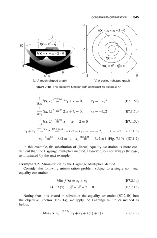
Figure 7.10 The objective function with constraint for Example 7.1.

∂ (7.2.3a)
l(x,λ) = 2x 1 + λ = 0, x 1 =−λ/2 (E7.1.5a)
∂x 1
∂ (7.2.3a)
l(x,λ) = 2x 2 + λ = 0, x 2 =−λ/2 (E7.1.5b)
∂x 2
∂ (7.2.3b)
l(x,λ) = x 1 + x 2 − 2 = 0 (E7.1.5c)
∂λ
(E7.1.5c) (E7.1.5a,b)
x 1 + x 2 = 2 → −λ/2 − λ/2 =−λ = 2, λ =−2 (E7.1.6)
(E7.1.5a) (E7.1.5b)
x 1 = −λ/2 = 1, x 2 = −λ/2 = 1 (Fig. 7.10) (E7.1.7)
In this example, the substitution of (linear) equality constraints is more con-
venient than the Lagrange multiplier method. However, it is not always the case,
as illustrated by the next example.

Example 7.2. Minimization by the Lagrange Multiplier Method.
Consider the following minimization problem subject to a single nonlinear
equality constraint:

(E7.2.1a)
Min f(x) = x 1 + x 2
2
2
s.t.h(x) = x + x − 2 = 0 (E7.2.1b)
1 2
Noting that it is absurd to substitute the equality constraint (E7.2.1b) into
the objective function (E7.2.1a), we apply the Lagrange multiplier method as
below.

(7.2.2) 2 2
Min l(x,λ) = x 1 + x 2 + λ(x + x ) (E7.2.3)
1
2