Page 414 - Applied Numerical Methods Using MATLAB

ELLIPTIC PDE 403
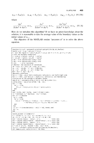
u i,0 = b x0 (y i ), u i,M x = b xf (y i ), u 0,j = b y0 (x j ), u M y ,j = b yf (x j ) (9.1.5b)

where
2
y 2 x 2 x y 2
= r y , = r x , = r xy (9.1.6)
2
2
2
2
2
2
2( x + y ) 2( x + y ) 2( x + y )
How do we initialize this algorithm? If we have no priori knowledge about the
solution, it is reasonable to take the average value of the boundary values as the
initial values of u i,j .
The objective of the MATLAB routine “poisson.m” is to solve the above
equation.
function [u,x,y] = poisson(f,g,bx0,bxf,by0,byf,D,Mx,My,tol,MaxIter)
%solve u_xx + u_yy + g(x,y)u = f(x,y)
% over the region D = [x0,xf,y0,yf] = {(x,y) |x0 <= x <= xf, y0 <= y <= yf}
% with the boundary Conditions:
% u(x0,y) = bx0(y), u(xf,y) = bxf(y)
% u(x,y0) = by0(x), u(x,yf) = byf(x)
%Mx=#of subintervals along x axis
%My=#of subintervals along y axis
% tol : error tolerance
% MaxIter: the maximum # of iterations
x0 = D(1); xf = D(2); y0 = D(3); yf = D(4);
dx = (xf - x0)/Mx; x = x0 + [0:Mx]*dx;
dy = (yf - y0)/My; y = y0 + [0:My]’*dy;
Mx1=Mx+1;My1=My + 1;
%Boundary conditions
for m = 1:My1, u(m,[1 Mx1])=[bx0(y(m)) bxf(y(m))]; end %left/right side
for n = 1:Mx1, u([1 My1],n) = [by0(x(n)); byf(x(n))]; end %bottom/top
%initialize as the average of boundary values
sum_of_bv = sum(sum([u(2:My,[1 Mx1]) u([1 My1],2:Mx)’]));
u(2:My,2:Mx) = sum_of_bv/(2*(Mx + My - 2));
for i = 1:My
for j = 1:Mx
F(i,j) = f(x(j),y(i)); G(i,j) = g(x(j),y(i));
end
end
dx2 = dx*dx; dy2 = dy*dy; dxy2 = 2*(dx2 + dy2);
rx = dx2/dxy2; ry = dy2/dxy2; rxy = rx*dy2;
for itr = 1:MaxIter
for j = 2:Mx
for i = 2:My
u(i,j) = ry*(u(i,j + 1)+u(i,j - 1)) + rx*(u(i + 1,j)+u(i - 1,j))...
+ rxy*(G(i,j)*u(i,j)- F(i,j)); %Eq.(9.1.5a)
end
end
if itr>1& max(max(abs(u - u0))) < tol, break; end
u0=u;
end
%solve_poisson in Example 9.1
f = inline(’0’,’x’,’y’); g = inline(’0’,’x’,’y’);
x0=0;xf=4;Mx= 20; y0=0;yf=4;My=20;
bx0 = inline(’exp(y) - cos(y)’,’y’); %(E9.1.2a)
bxf = inline(’exp(y)*cos(4) - exp(4)*cos(y)’,’y’); %(E9.1.2b)
by0 = inline(’cos(x) - exp(x)’,’x’); %(E9.1.3a)
byf = inline(’exp(4)*cos(x) - exp(x)*cos(4)’,’x’); %(E9.1.3b)
D = [x0 xf y0 yf]; MaxIter = 500; tol = 1e-4;
[U,x,y] = poisson(f,g,bx0,bxf,by0,byf,D,Mx,My,tol,MaxIter);
clf, mesh(x,y,U), axis([0 4 0 4 -100 100])