Page 418 - Applied Numerical Methods Using MATLAB

PARABOLIC PDE 407

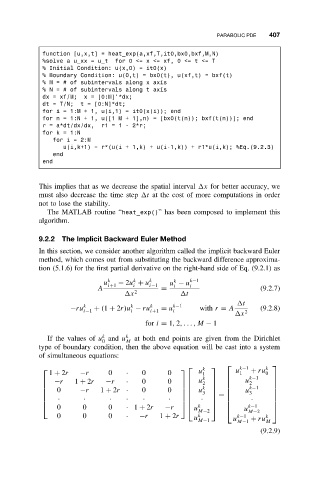
function [u,x,t] = heat_exp(a,xf,T,it0,bx0,bxf,M,N)
%solve a u_xx = u_t for 0 <= x <= xf, 0 <= t <= T
% Initial Condition: u(x,0) = it0(x)
% Boundary Condition: u(0,t) = bx0(t), u(xf,t) = bxf(t)
%M=#of subintervals along x axis
%N=#of subintervals along t axis
dx = xf/M; x = [0:M]’*dx;
dt = T/N; t = [0:N]*dt;
for i = 1:M + 1, u(i,1) = it0(x(i)); end
for n = 1:N + 1, u([1 M + 1],n) = [bx0(t(n)); bxf(t(n))]; end
r = a*dt/dx/dx, r1 = 1 - 2*r;
for k = 1:N
for i = 2:M
u(i,k+1) = r*(u(i + 1,k) + u(i-1,k)) + r1*u(i,k); %Eq.(9.2.3)
end
end

This implies that as we decrease the spatial interval x for better accuracy, we
must also decrease the time step t at the cost of more computations in order
not to lose the stability.
The MATLAB routine “heat_exp()” has been composed to implement this
algorithm.

9.2.2 The Implicit Backward Euler Method
In this section, we consider another algorithm called the implicit backward Euler
method, which comes out from substituting the backward difference approxima-
tion (5.1.6) for the first partial derivative on the right-hand side of Eq. (9.2.1) as
k
k
u k i+1 − 2u + u k i−1 u − u k−1
i
A = i i (9.2.7)
x 2 t
t
k−1
k
k
k
−ru + (1 + 2r)u − ru = u with r = A (9.2.8)
i−1 i i+1 i 2
x
for i = 1, 2,...,M − 1
k
If the values of u and u k at both end points are given from the Dirichlet
0 M
type of boundary condition, then the above equation will be cast into a system
of simultaneous equations:
 
 k  k−1 k
1 + 2r −r 0 · 0 0 1 1 0
  u u + ru
 −r 1 + 2r −r · 0 0   u k   u k−1 
2


 2  k−1
0 −r 1 + 2r · 0 0  u k  u
   
   3 
 3 
  =  
· · · · · ·  ·  ·
   
 
0 0 0 · 1 + 2r −r  u  u
  k  k−1 
M−2  M−2 
0 0 0 · −r 1 + 2r u k k−1 k
M−1 u M−1 + ru M
(9.2.9)