Page 420 - Applied Numerical Methods Using MATLAB

PARABOLIC PDE 409
9.2.3 The Crank–Nicholson Method
Here, let us go back to see Eq. (9.2.7) and try to improve the implicit backward
Euler method. The difference approximation on the left-hand side is taken at
time point k, while the difference approximation on the right-hand side is taken
at the midpoint between time k and k − 1, if we regard it as the central differ-
ence approximation with time step t/2. Doesn’t this seem to be inconsistent?
How about taking the difference approximation of both sides at the same time
point—say, the midpoint between k + 1and k—for balance? In order to do so,
we take the average of the central difference approximations of the left-hand side
at the two points k + 1and k, yielding

k+1 k+1 k+1 k k k k+1 k
A u i+1 − 2u i + u i−1 u i+1 − 2u + u i−1 u i − u i
i
+ = (9.2.15)
2 x 2 x 2 t
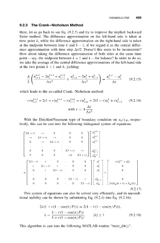
which leads to the so-called Crank–Nicholson method:

k+1 k+1 k+1 k k k
−ru + 2(1 + r)u − ru = ru + 2(1 − r)u + ru (9.2.16)
i+1 i i−1 i+1 i i−1
t
with r = A
x 2
With the Dirichlet/Neumann type of boundary condition on x 0 /x M , respec-
tively, this can be cast into the following tridiagonal system of equations.

 k+1 
  u
2(1 + r) −r 0 · 0 0 1

−r 2(1 + r) −r 0 0 
   u k+1 
 ·  2
 
  
 0 −r 2(1 + r) · 0 0   u k+1 
  3 
 
 
· · · · · ·  · 
 
 
 
 
0 0 0 · 2(1 + r) −r  k+1 
 
   u M−1 
0 0 0 · −2r 2(1 + r) u k+1
M
2(1 − r) r 0 · 0 0 u r(u + u )
   k   k+1 k 
1 0 0
r 2(1 − r) r · 0 0   u 0
   k   
2 
  
     
 0 r 2(1 − r) · 0 0   u k   0 
 
 3   
=     +  
· · · · · · · ·
     
     
0 0 0 · 2(1 − r) r   u 0
   k   
 M−1   
0 0 0 · 2r 2(1 − r) u k M 2r(b (k + 1) + b (k))

M
M
(9.2.17)
This system of equations can also be solved very efficiently, and its uncondi-
tional stability can be shown by substituting Eq. (9.2.4) into Eq. (9.2.16):
2λ(1 + r(1 − cos(π/P ))) = 2(1 − r(1 − cos(π/P ))),
1 − r(1 − cos(π/P ))
λ = , |λ|≤ 1 (9.2.18)
1 + r(1 − cos(π/P ))
This algorithm is cast into the following MATLAB routine “heat_CN()”.