Page 419 - Applied Numerical Methods Using MATLAB

408 PARTIAL DIFFERENTIAL EQUATIONS
How about the case where the values of ∂u/∂x| x=0 = b (t) at one end are

0
given? In that case, we approximate this Neumann type of boundary condition by
k
u − u k
1 −1
= b (k) (9.2.10)
0
2 x
and mix it up with one more equation associated with the unknown variable u k
0
k
k
−ru k + (1 + 2r)u − ru = u k−1 (9.2.11)
−1 0 1 0
to get
k k k−1

(1 + 2r)u − 2ru = u − 2rb (k) x (9.2.12)
0 1 0 0
We augment Eq. (9.2.9) with this to write
 k−1 
1 + 2r −2r 0 0 · 0 0 u 0 0 0
   k  u − 2rb (k) x
 −r 1 + 2r −r 0 · 0 0   u k   u k−1 

1


1 
 
 
0 −r 1 + 2r −r · 0 0   u  u 
   k  k−1
 2   2 
     k−1 
0 0 −r 1 + 2r 0 0   u k 
 · u
   3  =  3 
 
   
· · · · · · · ·  · 
   
 
0 0 0 1 + 2r −r   u  k−1 
   k 
 · · M−2  u
M−2 

0 0 0 · · −r 1 + 2r u k k−1 k
M−1 u + ru
M−1 M
(9.2.13)
Equations such as Eq. (9.2.9) or (9.2.13) are really nice in the sense that they
can be solved very efficiently by exploiting their tridiagonal structures and are
guaranteed to be stable owing to their diagonal dominancy. The unconditional
stability of Eq. (9.2.9) can be shown by substituting Eq. (9.2.4) into Eq. (9.2.8):
1
−jπ/P jπ/P
−re + (1 + 2r) − re = 1/λ, λ = , |λ|≤ 1
1 + 2r(1 − cos(π/P ))
(9.2.14)
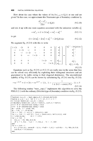
The following routine “heat_imp()” implements this algorithm to solve the
PDE (9.2.1) with the ordinary (Dirichlet type of) boundary condition via Eq. (9.2.9).
function [u,x,t] = heat_imp(a,xf,T,it0,bx0,bxf,M,N)
%solve a u_xx = u_t for 0 <= x <= xf, 0 <= t <= T
% Initial Condition: u(x,0) = it0(x)
% Boundary Condition: u(0,t) = bx0(t), u(xf,t) = bxf(t)
%M=#of subintervals along x axis
%N=#of subintervals along t axis
dx = xf/M; x = [0:M]’*dx;
dt = T/N; t = [0:N]*dt;
for i = 1:M + 1, u(i,1) = it0(x(i)); end
for n = 1:N + 1, u([1 M + 1],n) = [bx0(t(n)); bxf(t(n))]; end
r = a*dt/dx/dx; r2 = 1 + 2*r;
fori=1:M-1
A(i,i) = r2; %Eq.(9.2.9)
ifi>1,A(i- 1,i) = -r; A(i,i - 1) = -r; end
end
fork=2:N+1
b = [r*u(1,k); zeros(M - 3,1); r*u(M + 1,k)] + u(2:M,k - 1); %Eq.(9.2.9)
u(2:M,k) = trid(A,b);
end