Page 421 - Applied Numerical Methods Using MATLAB

410 PARTIAL DIFFERENTIAL EQUATIONS

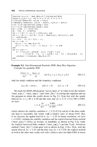
function [u,x,t] = heat_CN(a,xf,T,it0,bx0,bxf,M,N)
%solve a u_xx = u_t for 0 <= x <= xf, 0 <= t <= T
% Initial Condition: u(x,0) = it0(x)
% Boundary Condition: u(0,t) = bx0(t), u(xf,t) = bxf(t)
%M=#of subintervals along x axis
%N=#of subintervals along t axis
dx = xf/M; x = [0:M]’*dx;
dt = T/N; t = [0:N]*dt;
for i = 1:M + 1, u(i,1) = it0(x(i)); end
for n = 1:N + 1, u([1 M + 1],n) = [bx0(t(n)); bxf(t(n))]; end
r = a*dt/dx/dx;
r1 = 2*(1 - r); r2 = 2*(1 + r);
fori=1:M-1
A(i,i) = r1; %Eq.(9.2.17)
ifi>1,A(i- 1,i) = -r; A(i,i - 1) = -r; end
end
fork=2:N+1
b = [r*u(1,k); zeros(M - 3,1); r*u(M + 1,k)] ...
+ r*(u(1:M - 1,k - 1) + u(3:M + 1,k - 1)) + r2*u(2:M,k - 1);
u(2:M,k) = trid(A,b); %Eq.(9.2.17)
end

Example 9.2. One-Dimensional Parabolic PDE: Heat Flow Equation.
Consider the parabolic PDE

2
∂ u(x, t) ∂u(x, t)
= for 0 ≤ x ≤ 1, 0 ≤ t ≤ 0.1 (E9.2.1)
∂x 2 ∂t
with the initial condition and the boundary conditions

u(x, 0) = sin πx, u(0,t) = 0, u(1,t) = 0 (E9.2.2)

We made the MATLAB program “solve_heat.m” in order to use the routines
“heat_exp()”, “heat_imp()”, and “heat_CN()” in solving this equation and ran
this program to obtain the results shown in Fig. 9.3. Note that with the spatial
interval x = x f /M = 1/20 and the time step t = T/N = 0.1/100 = 0.001,
we have
t 0.001
r = A = 1 = 0.4 (E9.2.3)
x 2 (1/20) 2
which satisfies the stability condition (r ≤ 1/2) (9.2.6) and all of the three meth-
ods lead to reasonably fair results with a relative error of about 0.013. But,
if we decrease the spatial interval to x = 1/25 for better resolution, we have
r = 0.625, violating the stability condition and the explicit forward Euler method
(“heat_exp()”) blows up because of instability as shown in Fig. 9.3a, while
the implicit backward Euler method (“heat_imp()”) and the Crank–Nicholson
method (“heat_CN()”) work quite well as shown in Figs. 9.3b,c. Now, with the
spatial interval x = 1/25 and the time step t = 0.1/120, the explicit method
as well as the other ones works well with a relative error less than 0.001 in return