Page 425 - Applied Numerical Methods Using MATLAB

414 PARTIAL DIFFERENTIAL EQUATIONS

100

0

−100
4
y x 4
2 3
2
1
0 0
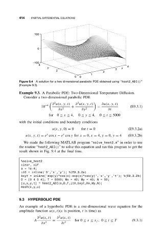
Figure 9.4 A solution for a two dimensional parabolic PDE obtained using ‘‘heat2 ADI()’’
(Example 9.3).
Example 9.3. A Parabolic PDE: Two-Dimensional Temperature Diffusion.
Consider a two-dimensional parabolic PDE

2 2
∂ u(x, y, t) ∂ u(x, y, t) ∂u(x,y,t)
−4
10 + = (E9.3.1)
∂x 2 ∂y 2 ∂t
for 0 ≤ x ≤ 4, 0 ≤ y ≤ 4, 0 ≤ t ≤ 5000
with the initial conditions and boundary conditions
u(x, y, 0) = 0 for t = 0 (E9.3.2a)
x
y
u(x, y, t) = e cos x − e cos y for x = 0,x = 4,y = 0,y = 4 (E9.3.2b)
We made the following MATLAB program “solve_heat2.m”in order to use
the routine “heat2_ADI()” to solve this equation and ran this program to get the
result shown in Fig. 9.4 at the final time.

%solve_heat2
clear, clf
a = 1e-4;
it0 = inline(’0’,’x’,’y’); %(E9.3.2a)
bxyt = inline(’exp(y)*cos(x)-exp(x)*cos(y)’,’x’,’y’,’t’); %(E9.3.2b)
D = [0 4 0 4]; T = 5000; Mx = 40; My = 40;N=50;
[u,x,y,t] = heat2_ADI(a,D,T,it0,bxyt,Mx,My,N);
mesh(x,y,u)

9.3 HYPERBOLIC PDE
An example of a hyperbolic PDE is a one-dimensional wave equation for the
amplitude function u(x, t)(x is position, t is time) as
2
2
∂ u(x, t) ∂ u(x, t)
A = for 0 ≤ x ≤ x f , 0 ≤ t ≤ T (9.3.1)
∂x 2 ∂t 2