Page 427 - Applied Numerical Methods Using MATLAB

416 PARTIAL DIFFERENTIAL EQUATIONS
We need the solution of this equation to be inside the unit circle for stability,
which requires
1 t 2
r ≤ , r = A ≤ 1 (9.3.7)
1 − cos(π/P ) x 2
The objective of the following MATLAB routine “wave()” is to implement
this algorithm for solving a one-dimensional wave equation.
Example 9.4. A Hyperbolic PDE: One-Dimensional Wave (Vibration). Consider
a one-dimensional hyperbolic PDE
2
2
∂ u(x, t) ∂u (x, t)
= for 0 ≤ x ≤ 2, 0 ≤ y ≤ 2, and 0 ≤ t ≤ 2 (E9.4.1)
∂x 2 ∂t 2
with the initial conditions and boundary conditions
u(x, 0) = x(1 − x), ∂u/∂t(x, 0) = 0 for t = 0 (E9.4.2a)
u(0,t) = 0 for x = 0, u(1,t) = 0 for x = 1 (E9.4.2b)

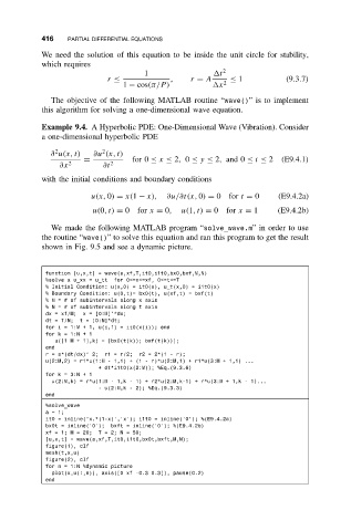
We made the following MATLAB program “solve_wave.m”inorder to use
the routine “wave()” to solve this equation and ran this program to get the result
shown in Fig. 9.5 and see a dynamic picture.

function [u,x,t] = wave(a,xf,T,it0,i1t0,bx0,bxf,M,N)
%solve a u_xx = u_tt for 0<=x<=xf, 0<=t<=T
% Initial Condition: u(x,0) = it0(x), u_t(x,0) = i1t0(x)
% Boundary Condition: u(0,t)= bx0(t), u(xf,t) = bxf(t)
%M=#of subintervals along x axis
%N=#of subintervals along t axis
dx = xf/M; x = [0:M]’*dx;
dt = T/N; t = [0:N]*dt;
for i = 1:M + 1, u(i,1) = it0(x(i)); end
fork=1:N+1
u([1 M + 1],k) = [bx0(t(k)); bxf(t(k))];
end
r = a*(dt/dx)^ 2; r1 = r/2; r2 = 2*(1 - r);
u(2:M,2) = r1*u(1:M - 1,1) + (1 - r)*u(2:M,1) + r1*u(3:M + 1,1) ...
+ dt*i1t0(x(2:M)); %Eq.(9.3.6)
fork=3:N+1
u(2:M,k) = r*u(1:M - 1,k - 1) + r2*u(2:M,k-1) + r*u(3:M + 1,k - 1)...
- u(2:M,k - 2); %Eq.(9.3.3)
end
%solve_wave
a=1;
it0 = inline(’x.*(1-x)’,’x’); i1t0 = inline(’0’); %(E9.4.2a)
bx0t = inline(’0’); bxft = inline(’0’); %(E9.4.2b)
xf=1;M=20; T=2;N=50;
[u,x,t] = wave(a,xf,T,it0,i1t0,bx0t,bxft,M,N);
figure(1), clf
mesh(t,x,u)
figure(2), clf
for n = 1:N %dynamic picture
plot(x,u(:,n)), axis([0 xf -0.3 0.3]), pause(0.2)
end