Page 428 - Applied Numerical Methods Using MATLAB

HYPERBOLIC PDE 417
0.3
0.2
0.2 0.1

0 0
−0.1
−0.2
1
2 −0.2
0.5 t
1 −0.3
0 0 0 0.2 0.4 0.6 0.8 x 1
(a) (b) A snap shot
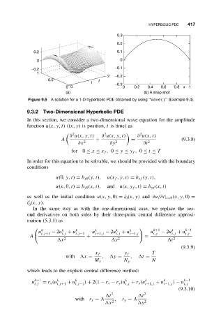
Figure 9.5 A solution for a 1-D hyperbolic PDE obtained by using ‘‘wave()’’ (Example 9.4).

9.3.2 Two-Dimensional Hyperbolic PDE
In this section, we consider a two-dimensional wave equation for the amplitude
function u(x, y, t) ((x, y) is position, t is time) as
2 2 2
∂ u(x, y, t) ∂ u(x, y, t) ∂ u(x, t)
A + = (9.3.8)
∂x 2 ∂y 2 ∂t 2
for 0 ≤ x ≤ x f , 0 ≤ y ≤ y f , 0 ≤ t ≤ T

In order for this equation to be solvable, we should be provided with the boundary
conditions

u(0,y,t) = b x0 (y, t), u(x f ,y, t) = b xf (y, t),
u(x, 0,t) = b y0 (x, t), and u(x, y f ,t) = b yf (x, t)

as well as the initial condition u(x, y, 0) = i 0 (x, y) and ∂u/∂t| t=0 (x, y, 0) =

i (x, y).
0
In the same way as with the one-dimensional case, we replace the sec-
ond derivatives on both sides by their three-point central difference approxi-
mation (5.3.1) as

k k k k k k k+1 k k−1
u i,j+1 − 2u i,j + u i,j−1 u i+1,j − 2u i,j + u i−1,j u i,j − 2u i,j + u i,j
A + =
x 2 y 2 t 2
(9.3.9)
x f y f T
with x = , y = , t =
M x N y N
which leads to the explicit central difference method:
k+1 k k k k k k−1
u = r x (u + u ) + 2(1 − r x − r y )u + r y (u + u ) − u
i,j i,j+1 i,j−1 i,j i+1,j i−1,j i,j
(9.3.10)
t 2 t 2
with r x = A , r y = A
x 2 y 2