Page 423 - Applied Numerical Methods Using MATLAB

412 PARTIAL DIFFERENTIAL EQUATIONS
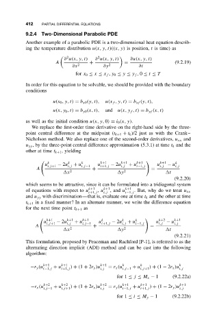
9.2.4 Two-Dimensional Parabolic PDE
Another example of a parabolic PDE is a two-dimensional heat equation describ-
ing the temperature distribution u(x, y, t)((x, y) is position, t is time) as
∂ u(x, y, t) ∂ u(x, y, t) ∂u(x, y, t)
2 2
A + = (9.2.19)
∂x 2 ∂y 2 ∂t
for x 0 ≤ x ≤ x f ,y 0 ≤ y ≤ y f , 0 ≤ t ≤ T

In order for this equation to be solvable, we should be provided with the boundary
conditions

u(x 0 ,y,t) = b x0 (y, t), u(x f ,y, t) = b xf (y, t),
u(x, y 0 ,t) = b y0 (x, t), and u(x, y f ,t) = b yf (x, t)

as well as the initial condition u(x, y, 0) = i 0 (x, y).
We replace the first-order time derivative on the right-hand side by the three-
point central difference at the midpoint (t k+1 + t k )/2 just as with the Crank–
Nicholson method. We also replace one of the second-order derivatives, u xx and
u yy , by the three-point central difference approximation (5.3.1) at time t k and the
other at time t k+1 , yielding

k k k k+1 k+1 k+1 k+1 k
u i,j+1 − 2u i,j + u i,j−1 u i+1,j − 2u i,j + u i−1,j u i,j − u i,j
A + =
x 2 y 2 t
(9.2.20)
which seems to be attractive, since it can be formulated into a tridiagonal system
of equations with respect to u k+1 , u k+1 ,and u k+1 . But, why do we treat u xx
i+1,j i,j i−1,j
and u yy with discrimination—that is, evaluate one at time t k and the other at time
t k+1 in a fixed manner? In an alternate manner, we write the difference equation
for the next time point t k+1 as

k+1 k+1 k+1 k k k k+2 k+1
u i,j+1 − 2u i,j + u i,j−1 u i+1,j − 2u i,j + u i−1,j u i,j − u i,j
A + =
x 2 y 2 t
(9.2.21)
This formulation, proposed by Peaceman and Rachford [P-1], is referred to as the
alternating direction implicit (ADI) method and can be cast into the following
algorithm:

−r y (u k+1 + u k+1 ) + (1 + 2r y )u k+1 = r x (u k + u k ) + (1 − 2r x )u k
i−1,j i+1,j i,j i,j−1 i,j+1 i,j
for 1 ≤ j ≤ M x − 1 (9.2.22a)
−r x (u k+2 + u k+2 ) + (1 + 2r x )u k+2 = r y (u k+1 + u k+1 ) + (1 − 2r y )u k+1
i,j−1 i,j+1 i,j i−1,j i+1,j i,j
for 1 ≤ i ≤ M y − 1 (9.2.22b)