Page 422 - Applied Numerical Methods Using MATLAB

PARABOLIC PDE 411

5 1

0 0.5

−5 0
1 1
x 0.1 x 0.1
t t
0.05 0.5 0.05
0 0 0 0
(a) The explicit method (b) The implicit method
1

0.5

0
1 x 0.1
0.5 0.05 t
0 0
(c) The Crank-Nicholson method
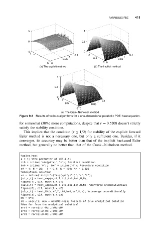
Figure 9.3 Results of various algorithms for a one-dimensional parabolic PDE: heat equation.
for somewhat (30%) more computations, despite that r = 0.5208 doesn’t strictly
satisfy the stability condition.
This implies that the condition (r ≤ 1/2) for stability of the explicit forward
Euler method is not a necessary one, but only a sufficient one. Besides, if it
converges, its accuracy may be better than that of the implicit backward Euler
method, but generally no better than that of the Crank–Nicholson method.

%solve_heat
a = 1; %the parameter of (E9.2.1)
it0 = inline(’sin(pi*x)’,’x’); %initial condition
bx0 = inline(’0’); bxf = inline(’0’); %boundary condition
xf = 1; M = 25; T = 0.1; N = 100; %r = 0.625
%analytical solution
uo = inline(’sin(pi*x)*exp(-pi*pi*t)’,’x’,’t’);
[u1,x,t] = heat_exp(a,xf,T,it0,bx0,bxf,M,N);
figure(1), clf, mesh(t,x,u1)
[u2,x,t] = heat_imp(a,xf,T,it0,bx0,bxf,M,N); %converge unconditionally
figure(2), clf, mesh(t,x,u2)
[u3,x,t] = heat_CN(a,xf,T,it0,bx0,bxf,M,N); %converge unconditionally
figure(3), clf, mesh(t,x,u3)
MN = M*N;
Uo = uo(x,t); aUo = abs(Uo)+eps; %values of true analytical solution
%How far from the analytical solution?
err1 = norm((u1-Uo)./aUo)/MN
err2 = norm((u2-Uo)./aUo)/MN
err3 = norm((u3-Uo)./aUo)/MN