Page 416 - Applied Numerical Methods Using MATLAB

ELLIPTIC PDE 405

u(x, y)
100

50

0

−50

−100
4
3 4
2 3
2
1
y 1 x
0 0
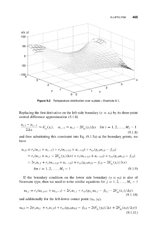
Figure 9.2 Temperature distribution over a plate—Example 9.1.

Replacing the first derivative on the left-side boundary (x = x 0 ) by its three-point
central difference approximation (5.1.8)

u i,1 − u i,−1
≈ b (y i ), u i,−1 ≈ u i,1 − 2b (y i ) x for i = 1, 2,...,M y − 1
2 x x 0 x 0
(9.1.8)
and then substituting this constraint into Eq. (9.1.5a) at the boundary points, we
have

u i,0 = r y (u i,1 + u i,−1 ) + r x (u i+1,0 + u i−1,0 ) + r xy (g i,0 u i,0 − f i,0 )

= r y (u i,1 + u i,1 − 2b (y i ) x) + r x (u i+1,0 + u i−1,0 ) + r xy (g i,0 u i,0 − f i,0 )
x 0

= 2r y u i,1 + r x (u i+1,0 + u i−1,0 ) + r xy (g i,0 u i,0 − f i,0 − 2b (y i )/ x)
x 0
for i = 1, 2,... ,M y − 1 (9.1.9)
If the boundary condition on the lower side boundary (y = y 0 )isalsoof
Neumann type, then we need to write similar equations for j = 1, 2,. ..,M x − 1

u 0,j = r y (u 0,j+1 + u 0,j−1 ) + 2r x u 1,j + r xy (g 0,j u 0,j − f 0,j − 2b (x j )/ y)
y 0
(9.1.10)
and additionally for the left-lower corner point (x 0 ,y 0 ),

u 0,0 = 2(r y u 0,1 + r x u 1,0 ) + r xy (g 0,0 u 0,0 − f 0,0 − 2(b (y 0 )/ x + 2b (x 0 )/ y))
x 0 y 0
(9.1.11)