Page 415 - Applied Numerical Methods Using MATLAB

404 PARTIAL DIFFERENTIAL EQUATIONS
Example 9.1. Laplace’s Equation—Steady-State Temperature Distribution.
Consider Laplace’s equation
2
2
∂ u(x, y) ∂ u(x, y)
2
∇ u(x, y) = + = 0 for 0 ≤ x ≤ 4, 0 ≤ y ≤ 4
∂x 2 ∂y 2
(E9.1.1)
with the boundary conditions
y
4
y
u(0,y) = e − cos y, u(4,y) = e cos 4 − e cos y (E9.1.2)
x
x
4
u(x, 0) = cos x − e , u(x, 4) = e cos x − e cos 4 (E9.1.3)
What we will get from solving this equation is u(x, y), which supposedly
describes the temperature distribution over a square plate having each side 4
units long (Fig. 9.1). We made the MATLAB program “solve_poisson.m”in
order to use the routine “poisson()” to solve Laplace’s equation given above
and run this program to obtain the result shown in Fig. 9.2.

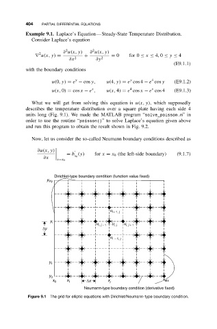
Now, let us consider the so-called Neumann boundary conditions described as

∂u(x, y)
= b (y) for x = x 0 (the left-side boundary) (9.1.7)
∂x x 0
x=x 0
Dirichlet-type boundary condition (function value fixed)
y My

u i + 1, j

y
i
u i, j − 1 u i, j u i, j + 1
∆y
u i − 1, j

y 1

y 0
x 0 x 1 ∆x x j x Mx
Neumann-type boundary condition (derivative fixed)

Figure 9.1 The grid for elliptic equations with Dirichlet/Neumann-type boundary condition.