Page 463 - Applied Numerical Methods Using MATLAB

452 PARTIAL DIFFERENTIAL EQUATIONS
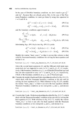
In the case of Dirichlet boundary condition, we don’t need to get u k+1
0
k+1
and u , because they are already given. But, in the case of the Neu-
M
mann boundary condition, we must get them by using this equation for
i = 0and M as
k
k
u k+1 = r(u + u ) + (1 − 2r)u k (P9.5.3a)
0 1 −1 0
u k+1 = r(u k + u k ) + (1 − 2r)u k (P9.5.3b)
M M+1 M−1 M
and the boundary conditions approximated as
k
u − u k
1 −1 k k
= b (k), u −1 = u − 2b (k) x (P9.5.4a)
0
0
1
2 x
u k − u k
M+1 M−1 k k
= b (k), u M+1 = u M−1 + 2b (k) x (P9.5.4b)
M
M
2 x
Substituting Eqs. (P9.5.4a,b) into Eq. (P9.5.3) yields
k+1 k k
u = 2r(u − b (k) x) + (1 − 2r)u (P9.5.5a)
0 1 0 0

u k+1 = 2r(u k + b (k) x) + (1 − 2r)u k (P9.5.5b)
M M−1 M M
Modify the routine “heat_exp()” so that it can use this scheme to deal
with the Neumann boundary conditions for solving the heat equation and
declare it as
function [u,x,t] = heat_exp_Neuman(a,xfn,T,it0,bx0,bxf,M,N)
where the second input argument xfn and the fifth and sixth input argu-

(t), b (t), respec-
ments bx0,bxf are supposed to carry [xf01] and b x 0
x f
tively, if the boundary condition at x 0 /x f is of Dirichlet/Neumann type and

they are also supposed to carry [xf 1 1] and b (t), b (t), respectively,

x 0 x f
if both of the boundary conditions at x 0 /x f are of Neumann type.
(b) Consider the implicit backward Euler algorithm described by Eq. (9.2.13),
which deals with the Neumann boundary condition at the one end for
solving the heat equation (9.2.1). With reference to Eq. (9.2.13), modify
the routine “heat_imp()” so that it can solve the heat equation with the
Neumann boundary conditions at two end points x 0 and x f and declare
it as
function [u,x,t] = heat_imp_Neuman(a,xfn,T,it0,bx0,bxf,M,N)
(c) Consider the Crank–Nicholson algorithm described by Eq. (9.2.17), which
deals with the Neumann boundary condition at the one end for solving the
heat equation (9.2.1). With reference to Eq. (9.2.17), modify the routine
“heat_cn()” so that it can solve the heat equation with the Neumann
boundary conditions at two end points x 0 and x f and declare it as

function [u,x,t] = heat_cn_Neuman(a,xfn,T,it0,bx0,bxf,M,N)