Page 83 - Applied Petroleum Geomechanics

74 Applied Petroleum Geomechanics

Detournay and Cheng (1993) used K (the drained bulk modulus of
elasticity) to replace K dry in the above equation for computing Biot’s
coefficient.
The dry bulk modulus can be related to dry Young’s modulus (E dry ) and
dry Poisson’s ratio (n dry ) as shown in the following equation:
E dry
K dry ¼ (2.78)
3ð1 2n dry Þ

The matrix bulk modulus (K m )isaconstant,depending on the
chemical composition of the minerals, e.g., for clay minerals K m varies
from 9.3 GPa in smectite up to >100 GPa in chlorite. When the
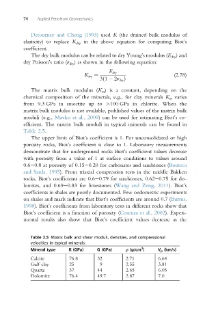
matrix bulk modulus is not available, published values of the matrix bulk
moduli (e.g., Mavko et al., 2009) can be used for estimating Biot’sco-
efficient. The matrix bulk moduli in typical minerals can be found in
Table 2.5.
The upper limit of Biot’s coefficient is 1. For unconsolidated or high
porosity rocks, Biot’s coefficient is close to 1. Laboratory measurements
demonstrate that for underground rocks Biot’s coefficient values decrease
with porosity from a value of 1 at surface conditions to values around
0.6e0.8 at porosity of 0.15e0.20 for carbonates and sandstones (Bouteca
and Sarda, 1995). From triaxial compression tests in the middle Bakken
rocks, Biot’s coefficients are 0.6e0.79 for sandstones, 0.62e0.75 for do-
lomites, and 0.69e0.83 for limestones (Wang and Zeng, 2011). Biot’s
coefficients in shales are poorly documented. Few oedometric experiments
on shales and marls indicate that Biot’s coefficients are around 0.7 (Burrus,
1998). Biot’s coefficients from laboratory tests in different rocks show that
Biot’s coefficient is a function of porosity (Cosenza et al., 2002). Experi-
mental results also show that Biot’s coefficient values decrease as the

Table 2.5 Matrix bulk and shear moduli, densities, and compressional
velocities in typical minerals.
3
Mineral type K (GPa) G (GPa) r (g/cm ) V p (km/s)
Calcite 76.8 32 2.71 6.64
Gulf clay 25 9 2.55 3.81
Quartz 37 44 2.65 6.05
Dolomite 76.4 49.7 2.87 7.0