Page 81 - Applied Petroleum Geomechanics

72 Applied Petroleum Geomechanics

2.6.3 The relationship of dynamic and static Poisson’s
ratios

Dynamic Poisson’s ratio can be calculated from the compressional and shear
velocities of the elastic wave (V p , V s ), i.e.,

1 2
ðV p =V s Þ 1
2
n d ¼ 2 (2.76)
ðV p =V s Þ 1
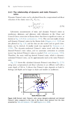
Laboratory measurements of static and dynamic Poisson’s ratios in
mudstones, siltstones, and siltstones with dolomites in the Chase and
Council Grove reservoirs in Kansas show that there is significant scatter, as
shown in Fig. 2.28 (Yale and Jamieson, 1994). The core test results of static
and dynamic Poisson’s ratios in the Baxter shale (Higgins et al., 2008) are
also plotted in Fig. 2.28, and the data are also scatter and no good corre-
lation can be derived. A similar result was reported by Tutuncu et al.
(1998). The dynamic-undrained Poisson’s ratios trend with the static-
drained Poisson’s ratio values, and no systematic correction to acoustic
(sonic) log derived Poisson’s ratios is needed (Yale and Jamieson, 1994).
Therefore, the sonic well log derived Poisson’s ratio, which is dynamic-
undrained Poisson’s ratio, can be approximately used as the static Poisson’s
ratio.
Fig. 2.29 shows the calculated dynamic Poisson’s ratio from Eq. (2.76)
using sonic compressional and shear velocities in an offshore well with a
water depth of 264 m. It shows that Poisson’s ratio depends on both li-
thology and depth and is larger in shales and smaller in sandstones.

0.4 Baxter shale: Higgins, 2008
Dynamic Poisson's ra o 0.2
Dynamic drained: Yale, 1994
Dynamic undrained: Yale, 1994
0.3

0.1

0
0 0.1 0.2 0.3 0.4
Sta c Poisson's ra o
Figure 2.28 Drained static Poisson’s ratio versus dynamic-undrained and drained
Poisson’s ratios compared to the data in the Baxter shale (plotted from the data
presented by Yale and Jamieson, 1994 and Higgins et al., 2008).