Page 259 - Applied Statistics And Probability For Engineers

PQ220 6234F.CD(06) 5/14/02 1:26 PM Page 1 RK UL 6 RK UL 6:Desktop Folder:TEMP WORK:MONTGOMERY:REVISES UPLO D CH114 FIN L:Quark F

6-8 MORE ABOUT PROBABILITY PLOTTING (CD ONLY)

Probability plots are extremely useful and are often the first technique used in an effort to
determine which probability distribution is likely to provide a reasonable model for the data.
We give a simple illustration of how a normal probability plot can be useful in distin-
guishing between normal and nonnormal data. Table S6-1 contains 50 observations gener-
ated at random from an exponential distribution with mean 20 (or 0.05 ). These data
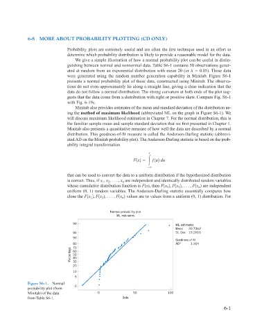
were generated using the random number generation capability in Minitab. Figure S6-1
presents a normal probability plot of these data, constructed using Minitab. The observa-
tions do not even approximately lie along a straight line, giving a clear indication that the
data do not follow a normal distribution. The strong curvature at both ends of the plot sug-
gests that the data come from a distribution with right or positive skew. Compare Fig. S6-1
with Fig. 6-19c.
Minitab also provides estimates of the mean and standard deviation of the distribution us-
ing the method of maximum likelihood (abbreviated ML on the graph in Figure S6-1). We
will discuss maximum likelihood estimation in Chapter 7. For the normal distribution, this is
the familiar sample mean and sample standard deviation that we first presented in Chapter 1.
Minitab also presents a quantitative measure of how well the data are described by a normal
distribution. This goodness-of-fit measure is called the Anderson-Darling statistic (abbrevi-
ated AD on the Minitab probability plot). The Anderson-Darling statistic is based on the prob-
ability integral transformation
x
F1x2 f 1u2 du

that can be used to convert the data to a uniform distribution if the hypothesized distribution
is correct. Thus, if x , x , . . . , x n are independent and identically distributed random variables
2
1
whose cumulative distribution function is F(x), then F1x 2, F1x 2, . . . , F1x 2 are independent
n
2
1
uniform (0, 1) random variables. The Anderson-Darling statistic essentially compares how
close the F1x 2, F1x 2, . . . , F1x 2 values are to values from a uniform (0, 1) distribution. For
1
2
n
Normal probability plot
ML estimates
99
ML estimates
Mean 20.7362
95 St. Dev. 19.2616
90
Goodness of fit
80 AD* 1.904
70
Percentage 60
50
40
30
20
10
5
Figure S6-1. Normal
0
probability plot (from
Minitab) of the data 0 50 100
from Table S6-1. Data

6-1