Page 256 - Applied Statistics And Probability For Engineers

c06.qxd 5/14/02 9:57 M Page 217 RK UL 6 RK UL 6:Desktop Folder:TEMP WORK:MONTGOMERY:REVISES UPLO D CH114 FIN L:Quark Files:

6-7 PROBABILITY PLOTS 217

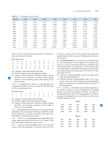
Table 6-7 Champagne Sales in France
Month 1962 1963 1964 1965 1966 1967 1968 1969
Jan. 2.851 2.541 3.113 5.375 3.633 4.016 2.639 3.934
Feb. 2.672 2.475 3.006 3.088 4.292 3.957 2.899 3.162
Mar. 2.755 3.031 4.047 3.718 4.154 4.510 3.370 4.286
Apr. 2.721 3.266 3.523 4.514 4.121 4.276 3.740 4.676
May 2.946 3.776 3.937 4.520 4.647 4.968 2.927 5.010
June 3.036 3.230 3.986 4.539 4.753 4.677 3.986 4.874
July 2.282 3.028 3.260 3.663 3.965 3.523 4.217 4.633
Aug. 2.212 1.759 1.573 1.643 1.723 1.821 1.738 1.659
Sept. 2.922 3.595 3.528 4.739 5.048 5.222 5.221 5.591
Oct. 4.301 4.474 5.211 5.428 6.922 6.873 6.424 6.981
Nov. 5.764 6.838 7.614 8.314 9.858 10.803 9.842 9.851
Dec. 7.132 8.357 9.254 10.651 11.331 13.916 13.076 12.670

batch of size 50. During 40 days of production, 40 batches of Construct a separate plot for each gasoline formulation, but
data were collected as follows: arrange the plots on the same axes. What tentative conclusions
can you draw?
Read data across.
6-84. Transformations. In some data sets, a transformation
9 12 6 9 7 14 12 4 6 7
by some mathematical function applied to the original data,
8 5 9 7 8 11 3 6 7 7
such as 1y or log y, can result in data that are simpler to work
11 4 4 8 7 5 6 4 5 8
with statistically than the original data. To illustrate the effect
19 19 18 12 11 17 15 17 13 13 of a transformation, consider the following data, which repre-
(a) Construct a stem-and-leaf plot of the data. sent cycles to failure for a yarn product: 675, 3650, 175, 1150,
(b) Find the sample average and standard deviation. 290, 2000, 100, 375.
(c) Construct a time series plot of the data. Is there evidence (a) Construct a normal probability plot and comment on the
that there was an increase or decrease in the average shape of the data distribution.
number of nonconforming springs made during the 40 (b) Transform the data using logarithms; that is, let y* (new
days? Explain. value) = log y (old value). Construct a normal probability
plot of the transformed data and comment on the effect of
6-80. A communication channel is being monitored by
recording the number of errors in a string of 1000 bits. Data the transformation.
for 20 of these strings follow: 6-85. In 1879, A. A. Michelson made 100 determinations of
the velocity of light in air using a modification of a method
Read data across. proposed by the French physicist Foucault. He made the
3 1 0 1 3 2 4 1 3 1 measurements in five trials of 20 measurements each. The ob-
1 1 2 3 3 2 0 2 0 1 servations (in kilometers per second) follow. Each value has
299,000 substracted from it.
(a) Construct a stem-and-leaf plot of the data.
(b) Find the sample average and standard deviation. Trial 1
(c) Construct a time series plot of the data. Is there evidence
that there was an increase or decrease in the number of 850 900 930 950 980
errors in a string? Explain. 1000 930 760 1000 960
6-81. Reconsider the data in Exercise 6-76. Construct normal 740 1070 850 980 880
probability plots for two groups of the data: the first 40 and the 980 650 810 1000 960
last 40 observations. Construct both plots on the same axes.
What tentative conclusions can you draw? Trial 2
6-82. Construct a normal probability plot of the effluent dis-
960 960 880 850 900
charge temperature data from Exercise 6-47. Based on the
830 810 880 800 760
plot, what tentative conclusions can you draw?
940 940 800 880 840
6-83. Construct normal probability plots of the cold start
790 880 830 790 800
ignition time data presented in Exercises 6-44 and 6-56.