Page 254 - Applied Statistics And Probability For Engineers

c06.qxd 5/14/02 9:56 M Page 215 RK UL 6 RK UL 6:Desktop Folder:TEMP WORK:MONTGOMERY:REVISES UPLO D CH114 FIN L:Quark Files:

6-7 PROBABILITY PLOTS 215

3.30 3.30 3.30

1.65 1.65 1.65

z z z
j 0 j 0 j 0

–1.65 –1.65 –1.65

–3.30 –3.30 –3.30
170 180 190 200 210 220 170 180 190 200 210 220 170 180 190 200 210 220
x ( j) x ( j) x ( j)
(a) (b) (c)
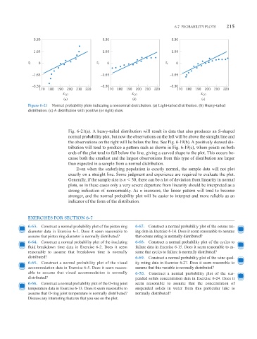
Figure 6-21 Normal probability plots indicating a nonnormal distrubution. (a) Light-tailed distribution. (b) Heavy-tailed
distribution. (c) A distribution with positive (or right) skew.

Fig. 6-21(a). A heavy-tailed distribution will result in data that also produces an S-shaped
normal probability plot, but now the observations on the left will be above the straight line and
the observations on the right will lie below the line. See Fig. 6-19(b). A positively skewed dis-
tribution will tend to produce a pattern such as shown in Fig. 6-19(c), where points on both
ends of the plot tend to fall below the line, giving a curved shape to the plot. This occurs be-
cause both the smallest and the largest observations from this type of distribution are larger
than expected in a sample from a normal distribution.
Even when the underlying population is exactly normal, the sample data will not plot
exactly on a straight line. Some judgment and experience are required to evaluate the plot.
Generally, if the sample size is n 30, there can be a lot of deviation from linearity in normal
plots, so in these cases only a very severe departure from linearity should be interpreted as a
strong indication of nonnormality. As n increases, the linear pattern will tend to become
stronger, and the normal probability plot will be easier to interpret and more reliable as an
indicator of the form of the distribution.

EXERCISES FOR SECTION 6-7

6-63. Construct a normal probability plot of the piston ring 6-67. Construct a normal probability plot of the octane rat-
diameter data in Exercise 6-1. Does it seem reasonable to ing data in Exercise 6-14. Does it seem reasonable to assume
assume that piston ring diameter is normally distributed? that octane rating is normally distributed?
6-64. Construct a normal probability plot of the insulating 6-68. Construct a normal probability plot of the cycles to
fluid breakdown time data in Exercise 6-2. Does it seem failure data in Exercise 6-15. Does it seem reasonable to as-
reasonable to assume that breakdown time is normally sume that cycles to failure is normally distributed?
distributed? 6-69. Construct a normal probability plot of the wine qual-
6-65. Construct a normal probability plot of the visual ity rating data in Exercise 6-27. Does it seem reasonable to
accommodation data in Exercise 6-5. Does it seem reason- assume that this variable is normally distributed?
able to assume that visual accommodation is normally 6-70. Construct a normal probability plot of the sus-
distributed? pended solids concentration data in Exercise 6-24. Does it
6-66. Construct a normal probability plot of the O-ring joint seem reasonable to assume that the concentration of
temperature data in Exercise 6-13. Does it seem reasonable to suspended solids in water from this particular lake is
assume that O-ring joint temperature is normally distributed? normally distributed?
Discuss any interesting features that you see on the plot.