Page 250 - Applied Statistics And Probability For Engineers

c06.qxd 5/14/02 9:55 M Page 211 RK UL 6 RK UL 6:Desktop Folder:TEMP WORK:MONTGOMERY:REVISES UPLO D CH114 FIN L:Quark Files:

6-6 TIME SEQUENCE PLOTS 211

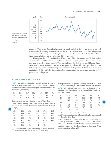
Leaf Stem Time series plot
8 9e
6 9s
45 9f
2333 9t
0010000 9z
99998 8e
Figure 6-18 A digi- 66677 8s
dot plot of chemical 45 8f
process concentration 23 8t
readings, observed 1 8z
hourly.

occurred. This plot effectively displays the overall variability in the compressive strength
data and simultaneously shows the variability in these measurements over time. The general
impression is that compressive strength varies around the mean value of 162.67, and there
is no strong obvious pattern in this variability over time.
The digidot plot in Fig. 6-18 tells a different story. This plot summarizes 30 observations
on concentration of the output product from a chemical process, where the observations are
recorded at one-hour time intervals. This plot indicates that during the first 20 hours of oper-
ation this process produced concentrations generally above 85 grams per liter, but that
following sample 20, something may have occurred in the process that results in lower con-
centrations. If this variability in output product concentration can be reduced, operation of this
process can be improved.

EXERCISES FOR SECTION 6-6

6-57. The College of Engineering and Applied Science at (b) Specifications on product viscosity are at 48 2. What
Arizona State University had a VAX computer system. conclusions can you make about process performance?
Response times for 20 consecutive jobs were recorded and are 6-59. The pull-off force for a connector is measured in a
as follows: (read across) laboratory test. Data for 40 test specimens follow (read down,
5.3 10.1 5.9 12.2 11.2 12.4 9.2 then left to right).
5.0 5.8 7.2 8.5 7.3 3.9 10.5 241 203 201 251 236 190
9.5 6.2 10.0 4.7 6.4 8.1 258 195 195 238 245 175
237 249 255 210 209 178
Construct and interpret a time series plot of these data.
210 220 245 198 212 175
6-58. The following data are the viscosity measurements
194 194 235 199 185 190
for a chemical product observed hourly (read down, then left
to right). 225 245 220 183 187
248 209 249 213 218
47.9 48.6 48.0 48.1 43.0 43.2
47.9 48.8 47.5 48.0 42.9 43.6 (a) Construct a time series plot of the data.
(b) Construct and interpret either a digidot plot or a stem-and-
48.6 48.1 48.6 48.3 43.6 43.2
leaf plot of the data.
48.0 48.3 48.0 43.2 43.3 43.5
6-60. In their book Time Series Analysis, Forecasting, and
48.4 47.2 47.9 43.0 43.0 43.0
Control (Prentice Hall, 1994), G. E. P. Box, G. M. Jenkins,
48.1 48.9 48.3 43.5 42.8
and G. C. Reinsel present chemical process concentration
48.0 48.6 48.5 43.1 43.1
readings made every two hours. Some of these data follow
(a) Construct and interpret either a digidot plot or a separate (read down, then left to right).
stem-and-leaf and time series plot of these data.