Page 253 - Applied Statistics And Probability For Engineers

c06.qxd 5/14/02 9:56 M Page 214 RK UL 6 RK UL 6:Desktop Folder:TEMP WORK:MONTGOMERY:REVISES UPLO D CH114 FIN L:Quark Files:

214 CHAPTER 6 RANDOM SAMPLING AND DATA DESCRIPTION

99.9 0.1
Table 6-6 Calculation for Constracting a Normal
99 1 Probability Plot
95 5 j x 1 j 2 1 j 0.52 10 z j
j – 0.5)/n 80 20 j – 0.5)/n] 1 2 176 0.05 1.64
0.15
183
1.04
50
50
100( 20 80 100[1 – ( 3 4 185 0.25 0.67
0.39
190
0.35
5 95 5 191 0.45 0.13
6 192 0.55 0.13
1 99
7 201 0.65 0.39
0.1 99.9 8 205 0.75 0.67
170 180 190 200 210 220
9 214 0.85 1.04
x ( j)
10 220 0.95 1.64
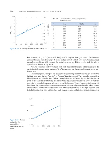
Figure 6-19 Normal probability plot for battery life.
For example, if 1 j 0.52 n 0.05, 1z 2 0.05 implies that z 1.64. To illustrate,
j
j
consider the data from Example 6-4. In the last column of Table 6-6 we show the standarized
normal scores. Figure 6-20 presents the plot of versus x 1 j2. This normal probability plot is
z
j
equivalent to the one in Fig. 6-19.
We have constructed our probability plots with the probability scale (or the z-scale) on the
vertical axis. Some computer packages “flip” the axis and put the probability scale on the hor-
izontal axis.
The normal probability plot can be useful in identifying distributions that are symmetric
but that have tails that are “heavier” or “lighter” than the normal. They can also be useful in
identifying skewed distributions. When a sample is selected from a light-tailed distribution
(such as the uniform distribution), the smallest and largest observations will not be as extreme
as would be expected in a sample from a normal distribution. Thus if we consider the straight
line drawn through the observations at the center of the normal probability plot, observations
on the left side will tend to fall below the line, whereas observations on the right side will tend
to fall above the line. This will produce an S-shaped normal probability plot such as shown in

3.30

1.65

z j
0

–1.65
Figure 6-20 Normal
probability plot
obtained from –3.30
standardized normal 170 180 190 200 210 220
scores. x ( j)