Page 275 - Applied Statistics And Probability For Engineers

c07.qxd 5/15/02 10:18 M Page 233 RK UL 6 RK UL 6:Desktop Folder:TEMP WORK:MONTGOMERY:REVISES UPLO D CH114 FIN L:Quark Files:

7-3 METHODS OF POINT ESTIMATION 233

Now

d ln L1 2 n n
a x i
d i 1
and upon equating this last result to zero we obtain

n
ˆ
n a X 1 X
i
i 1
Thus the maximum likelihood estimator of is the reciprocal of the sample mean. Notice that
this is the same as the moment estimator.

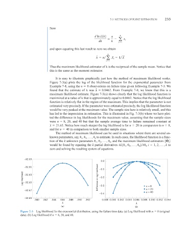
It is easy to illustrate graphically just how the method of maximum likelihood works.
Figure 7-3(a) plots the log of the likelihood function for the exponential parameter from
Example 7-8, using the n 8 observations on failure time given following Example 7-3. We
ˆ
found that the estimate of was 0.0462 . From Example 7-8, we know that this is a
maximum likelihood estimate. Figure 7-3(a) shows clearly that the log likelihood function is
maximized at a value of that is approximately equal to 0.0462. Notice that the log likelihood
function is relatively flat in the region of the maximum. This implies that the parameter is not
estimated very precisely. If the parameter were estimated precisely, the log likelihood function
would be very peaked at the maximum value. The sample size here is relatively small, and this
has led to the imprecision in estimation. This is illustrated in Fig. 7-3(b) where we have plot-
ted the difference in log likelihoods for the maximum value, assuming that the sample sizes
were n 8, 20, and 40 but that the sample average time to failure remained constant at
x 21.65 . Notice how much steeper the log likelihood is for n 20 in comparsion to n 8,
and for n 40 in comparison to both smaller sample sizes.
The method of maximum likelihood can be used in situations where there are several un-
k
2
known parameters, say, 1 , , p , to estimate. In such cases, the likelihood function is a func-
ˆ
tion of the k unknown parameters , , p , , and the maximum likelihood estimators 5 6
1
i
2
k
would be found by equating the k partial derivatives L1 , , p , 2 , i 1, 2, p , k to
2
1
i
k
zero and solving the resulting system of equations.
–32.59
0.0
–32.61 –0.1
Log likelihood –32.63 Difference in log likelihood –0.2
–32.65
n = 20
–32.67 –0.3 n = 8
n = 40
–0.4
–32.69
.040 .042 .044 .046 .048 .050 .052 0.038 0.040 0.042 0.044 0.046 0.048 0.050 0.052 0.054
λ λ
(a) (b)
Figure 7-3 Log likelihood for the exponential distribution, using the failure time data. (a) Log likelihood with n 8 (original
data). (b) Log likelihood if n 8, 20, and 40.