Page 355 - Applied Statistics And Probability For Engineers

c09.qxd 5/16/02 4:15 PM Page 303 RK UL 6 RK UL 6:Desktop Folder:TEMP WORK:MONTGOMERY:REVISES UPLO D CH114 FIN L:Quark Files:

9-3 TESTS ON THE MEAN OF A NORMAL DISTRIBUTION, VARIANCE UNKNOWN 303

7. Computations: Since x 0.83725 , s 0.02456, 0.82, and n 15, we have
0
0.83725 0.82
t 2.72
0
0.02456
115
8. Conclusions: Since t 2.72 1.761 , we reject H and conclude at the 0.05 level of
0
0
significance that the mean coefficient of restitution exceeds 0.82.
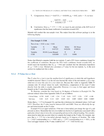
Minitab will conduct the one-sample t-test. The output from this software package is in the
following display:

One-Sample T: COR
Test of mu 0.82 vs mu 0.82
Variable N Mean StDev SE Mean
COR 15 0.83725 0.02456 0.00634
Variable 95.0% Lower Bound T P
COR 0.82608 2.72 0.008

Notice that Minitab computes both the test statistic T 0 and a 95% lower confidence bound for
the coefficient of restitution. Because the 95% lower confidence bound exceeds 0.82, we
would reject the hypothesis that H 0 : 0.82 and conclude that the alternative hypothesis
H : 0.82 is true. Minitab also calculates a P-value for the test statistic T 0 . In the next
1
section we explain how this is done.

9-3.2 P-Value for a t-Test

The P-value for a t-test is just the smallest level of significance at which the null hypothesis
would be rejected. That is, it is the tail area beyond the value of the test statistic t 0 for a one-
sided test or twice this area for a two-sided test. Because the t-table in Appendix Table IV
contains only 10 critical values for each t distribution, computation of the exact P-value
directly from the table is usually impossible. However, it is easy to find upper and lower
bounds on the P-value from this table.
To illustrate, consider the t-test based on 14 degrees of freedom in Example 9-6. The
relevant critical values from Appendix Table IV are as follows:
Critical Value: 0.258 0.692 1.345 1.761 2.145 2.624 2.977 3.326 3.787 4.140
Tail Area: 0.40 0.25 0.10 0.05 0.025 0.01 0.005 0.0025 0.001 0.0005

Notice that t 0 2.72 in Example 9-6, and that this is between two tabulated values, 2.624 and
2.977. Therefore, the P-value must be between 0.01 and 0.005. These are effectively the up-
per and lower bounds on the P-value.
Example 9-6 is an upper-tailed test. If the test is lower-tailed, just change the sign of t 0 and
proceed as above. Remember that for a two-tailed test the level of significance associated with a
particular critical value is twice the corresponding tail area in the column heading. This consider-
ation must be taken into account when we compute the bound on the P-value. For example, sup-
pose that t 0 2.72 for a two-tailed alternate based on 14 degrees of freedom. The value
t 2.624 (corresponding to 0.02) and t 0 2.977 (corresponding to 0.01), so the
0
lower and upper bounds on the P-value would be 0.01 P 0.02 for this case.