Page 84 - Applied Statistics And Probability For Engineers

PQ220 6234F.Ch 03 13/04/2002 03:19 PM Page 62

62 CHAPTER 3 DISCRETE RANDOM VARIABLES AND PROBABILITY DISTRIBUTIONS

f (x)
0.6561
Loading

0.2916 0.0036
0.0001
0.0486
0 1 2 3 4 x x
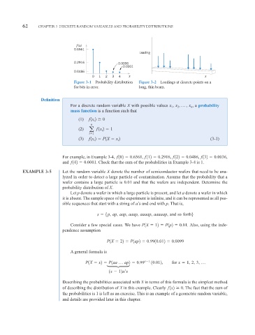
Figure 3-1 Probability distribution Figure 3-2 Loadings at discrete points on a
for bits in error. long, thin beam.

Definition
For a discrete random variable X with possible values x , x , p , x n , a probability
2
1
mass function is a function such that
(1) f 1x 2 0
i
n
(2) a f 1x 2 1
i
i 1
(3) f 1x 2 P1X x 2 (3-1)
i
i
For example, in Example 3-4, f 102 0.6561, f 112 0.2916, f 122 0.0486, f 132 0.0036,
and f 142 0.0001. Check that the sum of the probabilities in Example 3-4 is 1.

EXAMPLE 3-5 Let the random variable X denote the number of semiconductor wafers that need to be ana-
lyzed in order to detect a large particle of contamination. Assume that the probability that a
wafer contains a large particle is 0.01 and that the wafers are independent. Determine the
probability distribution of X.
Let p denote a wafer in which a large particle is present, and let a denote a wafer in which
it is absent. The sample space of the experiment is infinite, and it can be represented as all pos-
sible sequences that start with a string of a’s and end with p. That is,

s 5 p, ap, aap, aaap, aaaap, aaaaap, and so forth6

Consider a few special cases. We have P1X 12 P1p2 0.01. Also, using the inde-
pendence assumption

P1X 22 P1ap2 0.9910.012 0.0099
A general formula is

P1X x2 P1aa p ap2 0.99 x 1 10.012, for x 1, 2, 3, p
µ
1x 12a’s

Describing the probabilities associated with X in terms of this formula is the simplest method
of describing the distribution of X in this example. Clearly f 1x2 0 . The fact that the sum of
the probabilities is 1 is left as an exercise. This is an example of a geometric random variable,
and details are provided later in this chapter.