Page 25 - Applied statistics and probability for engineers

Section 1-1/The Engineering Method and Statistical Thinking 3

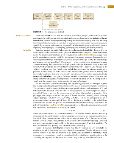
Develop a Identify the Propose or Manipulate Confirm Conclusions
clear important refine a the the and
description factors model model solution recommendations

Conduct
experiments

FIGURE 1-1 The engineering method.
The Science of Data The ield of statistics deals with the collection, presentation, analysis, and use of data to make
decisions, solve problems, and design products and processes. In simple terms, statistics is the sci-
ence of data. Because many aspects of engineering practice involve working with data, obviously
knowledge of statistics is just as important to an engineer as are the other engineering sciences.
Speciically, statistical techniques can be powerful aids in designing new products and systems,
improving existing designs, and designing, developing, and improving production processes.
Variability Statistical methods are used to help us describe and understand variability. By variability, we
mean that successive observations of a system or phenomenon do not produce exactly the same
result. We all encounter variability in our everyday lives, and statistical thinking can give us a
useful way to incorporate this variability into our decision-making processes. For example, con-
sider the gasoline mileage performance of your car. Do you always get exactly the same mileage
performance on every tank of fuel? Of course not — in fact, sometimes the mileage performance
varies considerably. This observed variability in gasoline mileage depends on many factors, such
as the type of driving that has occurred most recently (city versus highway), the changes in the
vehicle’s condition over time (which could include factors such as tire inlation, engine com-
pression, or valve wear), the brand and/or octane number of the gasoline used, or possibly even
the weather conditions that have been recently experienced. These factors represent potential
sources of variability in the system. Statistics provides a framework for describing this vari-
ability and for learning about which potential sources of variability are the most important or
which have the greatest impact on the gasoline mileage performance.
We also encounter variability in dealing with engineering problems. For example, suppose
that an engineer is designing a nylon connector to be used in an automotive engine application.
The engineer is considering establishing the design speciication on wall thickness at 3 32 inch
but is somewhat uncertain about the effect of this decision on the connector pull-off force. If
the pull-off force is too low, the connector may fail when it is installed in an engine. Eight
prototype units are produced and their pull-off forces measured, resulting in the following
,
.
.
.
.
data (in pounds): 12 6 12 9 13 4 12 3 13 6 13 5 12 6 13 1 . As we anticipated, not all of
,
,
.
,
.
,
.
,
.
,
the prototypes have the same pull-off force. We say that there is variability in the pull-off force
measurements. Because the pull-off force measurements exhibit variability, we consider the
pull-off force to be a random variable. A convenient way to think of a random variable, say X,
that represents a measurement is by using the model
X 5m1e (1-1)
where m is a constant and e is a random disturbance. The constant remains the same with every
measurement, but small changes in the environment, variance in test equipment, differences
in the individual parts themselves, and so forth change the value of e. If there were no distur-
bances, e would always equal zero and X would always be equal to the constant m. However,
this never happens in the real world, so the actual measurements X exhibit variability. We
often need to describe, quantify, and ultimately reduce variability.
Figure 1-2 presents a dot diagram of these data. The dot diagram is a very useful plot for
displaying a small body of data—say, up to about 20 observations. This plot allows us to easily
see two features of the data: the location, or the middle, and the scatter or variability. When
the number of observations is small, it is usually dificult to identify any speciic patterns in the
variability, although the dot diagram is a convenient way to see any unusual data features.