Page 53 - Applied statistics and probability for engineers

Section 2-2/Interpretations and Axioms of Probability 31

Equally Likely
Outcomes Whenever a sample space consists of N possible outcomes that are equally likely, the
probability of each outcome is 1/N.

It is frequently necessary to assign probabilities to events that are composed of several
outcomes from the sample space. This is straightforward for a discrete sample space.

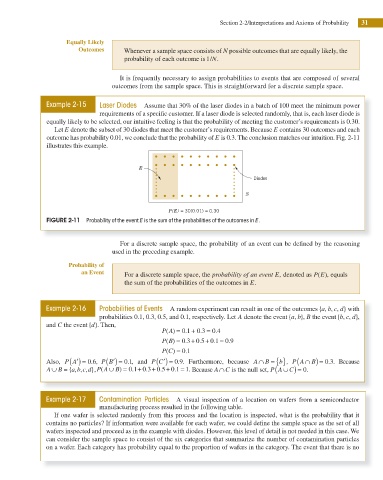
Example 2-15 Laser Diodes Assume that 30% of the laser diodes in a batch of 100 meet the minimum power
requirements of a speciic customer. If a laser diode is selected randomly, that is, each laser diode is

equally likely to be selected, our intuitive feeling is that the probability of meeting the customer’s requirements is 0.30.
Let E denote the subset of 30 diodes that meet the customer’s requirements. Because E contains 30 outcomes and each
outcome has probability 0.01, we conclude that the probability of E is 0.3. The conclusion matches our intuition. Fig. 2-11
illustrates this example.

E
Diodes

S

P(E) = 30(0.01) = 0.30
FIGURE 2-11 Probability of the event E is the sum of the probabilities of the outcomes in E.

For a discrete sample space, the probability of an event can be deined by the reasoning
used in the preceding example.
Probability of
an Event
For a discrete sample space, the probability of an event E, denoted as P E( ), equals
the sum of the probabilities of the outcomes in E.

b
c
Example 2-16 Probabilities of Events A random experiment can result in one of the outcomes { , , , } with
a
d
b
a
d
b
c
probabilities 0.1, 0.3, 0.5, and 0.1, respectively. Let A denote the event { , }, B the event { , , },
and C the event { }d . Then,
(
P A) = . + . = .0 1 0 3 0 4
(
P B) = . + . + . = .0 3 0 5 0 1 0 9
(
P C) = .0 1
b , (
(
Also, P A′ ( ) = .0 6 , P B′ = ) . 0 1, and P C′ ( ) = .9. Furthermore, because A∩ B = { } P A∩ B) = .3. Because
0
0
(
A∪ B = { a b c d}, P A( ∪ B) = 0 . + 0 . + 0 . + 0 . = 1 . Because A∩ C is the null set, P A∪ C) = 0.
5
1
1
3
,
,
,
Example 2-17 Contamination Particles A visual inspection of a location on wafers from a semiconductor
manufacturing process resulted in the following table.
If one wafer is selected randomly from this process and the location is inspected, what is the probability that it

contains no particles? If information were available for each wafer, we could deine the sample space as the set of all
wafers inspected and proceed as in the example with diodes. However, this level of detail is not needed in this case. We
can consider the sample space to consist of the six categories that summarize the number of contamination particles
on a wafer. Each category has probability equal to the proportion of wafers in the category. The event that there is no