Page 54 - Applied statistics and probability for engineers

32 Chapter 2/Probability

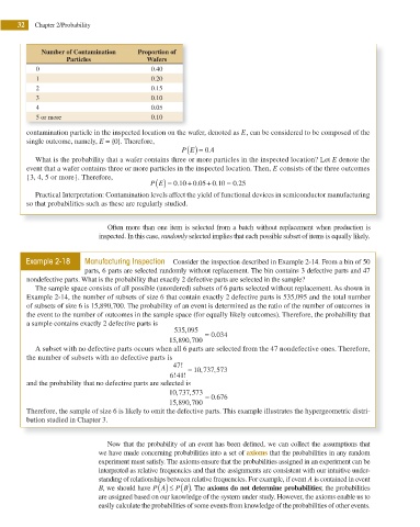
Number of Contamination Proportion of
Particles Wafers
0 0.40
1 0.20
2 0.15
3 0.10
4 0.05
5 or more 0.10
contamination particle in the inspected location on the wafer, denoted as E, can be considered to be composed of the
single outcome, namely, E = { }0 . Therefore,
0
P E ( ) = .4
What is the probability that a wafer contains three or more particles in the inspected location? Let E denote the
event that a wafer contains three or more particles in the inspected location. Then, E consists of the three outcomes
{3, 4, 5 or more}. Therefore,
0
P E ( ) = .0 10 + .05 + .10 = .25
0
0
Practical Interpretation: Contamination levels affect the yield of functional devices in semiconductor manufacturing
so that probabilities such as these are regularly studied.
Often more than one item is selected from a batch without replacement when production is
inspected. In this case, randomly selected implies that each possible subset of items is equally likely.

Example 2-18 Manufacturing Inspection Consider the inspection described in Example 2-14. From a bin of 50
parts, 6 parts are selected ran domly without replacement. The bin contains 3 defective parts and 47
nondefective parts. What is the probability that exactly 2 defective parts are selected in the sample?
The sample space consists of all possible (unordered) subsets of 6 parts selected without replacement. As shown in
Example 2-14, the number of subsets of size 6 that contain exactly 2 defective parts is 535,095 and the total number
of subsets of size 6 is 15,890,700. The probability of an event is determined as the ratio of the number of outcomes in
the event to the number of outcomes in the sample space (for equally likely outcomes). Therefore, the probability that
a sample contains exactly 2 defective parts is
535 095
,
= 0 034
.
,
,
15 890 700
A subset with no defective parts occurs when all 6 parts are selected from the 47 nondefective ones. Therefore,
the number of subsets with no defective parts is
47!
= 10 737 573
,
,
!
6 41!
and the probability that no defective parts are selected is
,
,
10 737 573
= 0 676
.
,
,
15 890 700
Therefore, the sample of size 6 is likely to omit the defective parts. This example illustrates the hypergeometric distri-
bution studied in Chapter 3.
Now that the probability of an event has been dei ned, we can collect the assumptions that
we have made concerning probabilities into a set of axioms that the probabilities in any random
experiment must satisfy. The axioms ensure that the probabilities assigned in an experiment can be
interpreted as relative frequencies and that the assignments are consistent with our intuitive under-
standing of relationships between relative frequencies. For example, if event A is contained in event
B, we should have P A ( ) ≤ (
P B). The axioms do not determine probabilities; the probabilities
are assigned based on our knowledge of the system under study. However, the axioms enable us to
easily calculate the probabilities of some events from knowledge of the probabilities of other events.