Page 121 - Artificial Intelligence for Computational Modeling of the Heart

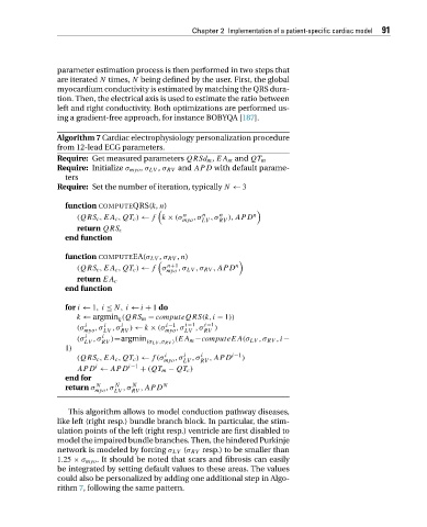
Chapter 2 Implementation of a patient-specific cardiac model 91

parameter estimation process is then performed in two steps that
are iterated N times, N being defined by the user. First, the global
myocardium conductivity is estimated by matching the QRS dura-
tion. Then, the electrical axis is used to estimate the ratio between
left and right conductivity. Both optimizations are performed us-
ing a gradient-free approach, for instance BOBYQA [187].

Algorithm 7 Cardiac electrophysiology personalization procedure
from 12-lead ECG parameters.
Require: Get measured parameters QRSd m , EA m and QT m
Require: Initialize σ myo , σ LV , σ RV and APD with default parame-
ters
Require: Set the number of iteration, typically N ← 3

function COMPUTEQRS(k, n)

(QRS c ,EA c ,QT c ) ← f k × (σ n ,σ n ,σ n ),APD n
myo LV RV
return QRS c
end function

function COMPUTEEA(σ LV , σ RV , n)

(QRS c ,EA c ,QT c ) ← f σ n+1 ,σ LV ,σ RV ,APD n
myo
return EA c
end function

for i ← 1,i ≤ N, i ← i + 1 do
k ← argmin (QRS m − computeQRS(k,i − 1))
k
i−1
i−1
i
i
i
i−1
(σ myo ,σ LV ,σ RV ) ← k × (σ myo ,σ LV ,σ RV )
(σ i ,σ i )=argmin (EA m −computeEA(σ LV ,σ RV ,i−
LV RV (σ LV ,σ RV )
1)
i
i
i
(QRS c ,EA c ,QT c ) ← f(σ myo ,σ LV ,σ RV ,APD i−1 )
i
APD ← APD i−1 + (QT m − QT c )
end for
N
N
N
return σ myo ,σ LV ,σ RV ,APD N
This algorithm allows to model conduction pathway diseases,
like left (right resp.) bundle branch block. In particular, the stim-
ulation points of the left (right resp.) ventricle are first disabled to
model the impaired bundle branches. Then, the hindered Purkinje
network is modeled by forcing σ LV (σ RV resp.) to be smaller than
1.25 × σ myo . It should be noted that scars and fibrosis can easily
be integrated by setting default values to these areas. The values
could also be personalized by adding one additional step in Algo-
rithm 7, following the same pattern.