Page 117 - Artificial Intelligence for Computational Modeling of the Heart

Chapter 2 Implementation of a patient-specific cardiac model 87

Figure 2.32. Cross-sectional flow variation with the peristaltic amplitude. An
excellent match with theory is obtained.

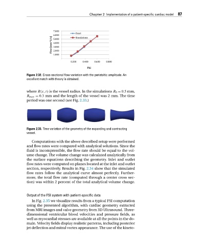
where R(x,t) is the vessel radius. In the simulations R 0 = 0.5 mm,
R max = 0.3 mm and the length of the vessel was 2 mm. The time
period was one second (see Fig. 2.33.)

Figure 2.33. Time variation of the geometry of the expanding and contracting
vessel.

Computations with the above described setup were performed
and flow rates were compared with analytical solutions. Since the
fluid is incompressible, the flow rate should be equal to the vol-
ume change. The volume change was calculated analytically from
the surface equations describing the geometry. Inlet and outlet
flow rates were computed on planes located at the inlet and outlet
section, respectively. Results in Fig. 2.34 show that the simulated
flow rates follow the analytical curve almost perfectly. Further-
more, the total flow rate (computed through a center cross sec-
tion) was within 2 percent of the total analytical volume change.

Output of the FSI system with patient-specific data
In Fig. 2.35 we visualize results from a typical FSI computation
using the presented algorithm, with cardiac geometry extracted
from MRI images and valve geometry from 3D Ultrasound. Three-
dimensional ventricular blood velocities and pressure fields, as
well as myocardial stresses are available at all the points in the do-
main. Velocity fields display realistic patterns, including posterior
jet deflection and mitral vortex appearance. The use of the kineto-