Page 115 - Artificial Intelligence for Computational Modeling of the Heart

Chapter 2 Implementation of a patient-specific cardiac model 85

Step 3
The third step runs the CFD solver using the new myocardial
wall and 3D valve positions. Here we discuss in detail the treat-
ment of the moving boundaries in LBM, which is of particular
interest for us, given the complex deformations encountered by
the endocardial wall and the cardiac valves. For lattice nodes lo-
cated near a boundary, i.e. where there is a neighboring node lo-
cated outside the fluid region, there are unknown f i values that are
required to complete the propagation step. The most commonly
used way to compute the unknown distributions is the bounce-
back approach: the unknown f i values, propagated from a solid
node, are set to the value corresponding to the opposite lattice
direction. This is equivalent to reversing the velocity of a particle
colliding with a static wall for example, f i = f j ,where c i =−c j are
two opposite lattice directions. For moving and curved walls one
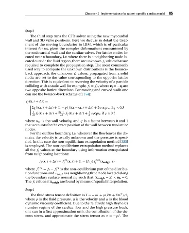
can use the bounce-back scheme of [254]:

f j (x,t + t) =

2qf i (x,t + t) + (1 − q)f i (x − c i ,t + t) + 2w i c j u w if q< 0.5
1 2q−1 1
q
2q f i (x,t + t) + 2q f j (x,t + t) + w i c j u w if q ≥ 0.5
where u w is the wall velocity, and q is a factor between 0 and 1
that accounts for the exact position of the wall between two lattice
nodes.
For the outflow boundary, i.e. wherever the flow leaves the do-
main, the velocity is usually unknown and the pressure is speci-
fied. In this case the non-equilibrium extrapolation method [255]
is employed. The non-equilibrium extrapolation method replaces
all the f i values at the boundary using information extrapolated
from neighboring locations:

eq neq
f j (x,t + t) = f (x,t) + (1 − Ω i,j )f (x ,t)
i i neigh
neq eq
where f = f i − f is the non-equilibrium part of the distribu-
i i
tion functions and x neigh is a neighboring fluid node located along
the boundary surface normal n such that (x neigh − x) × n = 0.
b
b
The f i values at x neigh are found by means of spatial interpolation.
Step 4
T
The fluid stress tensor definition is T =−pI + μ(∇u +∇u )/2,
where p is the fluid pressure, u is the velocity and μ is the blood
dynamic viscosity coefficient. Due to the relatively high Reynolds
number regime of the cardiac flow and the high pressure loads,
one can in a first approximation omit the contribution of the vis-
cous stress, and approximate the stress tensor as σ =−pI.The