Page 120 - Artificial Intelligence for Computational Modeling of the Heart

90 Chapter 2 Implementation of a patient-specific cardiac model

N
1 # 2
+ (p m [i]− p c [i]) . (2.38)
N
i=1
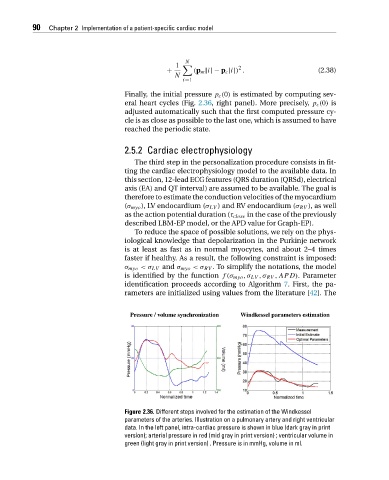
Finally, the initial pressure p c (0) is estimated by computing sev-
eral heart cycles (Fig. 2.36, right panel). More precisely, p c (0) is
adjusted automatically such that the first computed pressure cy-
cle is as close as possible to the last one, which is assumed to have
reached the periodic state.

2.5.2 Cardiac electrophysiology
The third step in the personalization procedure consists in fit-
ting the cardiac electrophysiology model to the available data. In
this section, 12-lead ECG features (QRS duration (QRSd), electrical
axis (EA) and QT interval) are assumed to be available. The goal is
therefore to estimate the conduction velocities of the myocardium
(σ myo ), LV endocardium (σ LV )and RVendocardium(σ RV ), as well
as the action potential duration (τ close in the case of the previously
described LBM-EP model, or the APD value for Graph-EP).
To reduce the space of possible solutions, we rely on the phys-
iological knowledge that depolarization in the Purkinje network
is at least as fast as in normal myocytes, and about 2–4 times
faster if healthy. As a result, the following constraint is imposed:
σ myo <σ LV and σ myo <σ RV . To simplify the notations, the model
is identified by the function f(σ myo ,σ LV ,σ RV ,APD). Parameter
identification proceeds according to Algorithm 7.First,the pa-
rameters are initialized using values from the literature [42]. The

Figure 2.36. Different steps involved for the estimation of the Windkessel
parameters of the arteries. Illustration on a pulmonary artery and right ventricular
data. In the left panel, intra-cardiac pressure is shown in blue (dark gray in print
version); arterial pressure in red (mid gray in print version) ; ventricular volume in
green (light gray in print version) . Pressure is in mmHg, volume in ml.