Page 119 - Artificial Intelligence for Computational Modeling of the Heart

Chapter 2 Implementation of a patient-specific cardiac model 89

2. Given the measured blood flow through the aortic and pul-
monary valves, as well as pressure information, estimate the
Windkessel parameters associated to the circulatory and pul-
monary systems respectively (section 2.5.1).
3. Given electrophysiology data, typically 12-lead ECG traces,
and the patient-specific anatomical model, estimate the elec-
trophysiology parameters (section 2.5.2).
4. Given measured volume curves, pressure information, along
with the personalized Windkessel and electrophysiology mod-
els, estimate the parameters of the biomechanical model (sec-
tion 2.5.3).
The following sections describe the optimization techniques
used to achieve each of these steps. AI-based methods for param-
eter estimations are presented in more details in chapter 5.

2.5.1 Windkessel parameters from pressure and
volume data
As described in section 1.4.1, arteries are modeled using a
Windkessel formulation. Model input is the blood through the
vessels. Model output is the resulting pressure curve, controlled by
the remote pressure, arterial compliance as well as characteristic
and peripheral resistances. The model also has an initial condition
to be estimated, namely the initial pressure.
Typically, one has at hand the flow curves through the arteries
(e.g. obtained from color Doppler ultrasound or magnetic reso-
nance imaging) and pressure information, either cuff pressure or
invasive catheterization. Let us assume that continuous pressure
and blood pool volume information are available. Both measure-
ments are often acquired at different time points, with different
heart rates and physiological conditions. Hence, a first step con-
sists in temporally aligning the volume and pressure curves. This
is achieved by first scaling the systolic portion of the pressure
curve such that the ejection time observed through the pressure
measurement matches the ejection time measured on the volume
curve. The diastolic phase is then matched by temporal stretching
(Fig. 2.36, left panel). Some low pass filtering may also be needed
to reduce the noise in the measurements.
The model parameters are then estimated automatically by
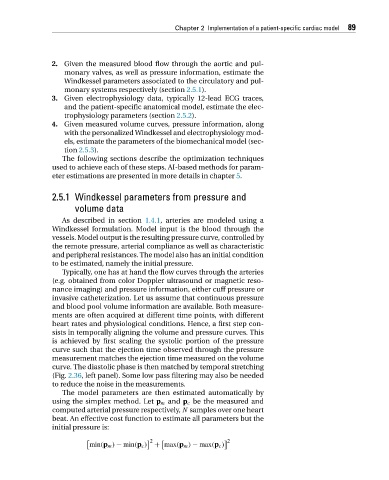
using the simplex method. Let p m and p c be the measured and
computed arterial pressure respectively, N samplesoverone heart
beat. An effective cost function to estimate all parameters but the
initial pressure is:

2 2

min(p m ) − min(p c ) + max(p m ) − max(p c )