Page 122 - Artificial Intelligence for Computational Modeling of the Heart

92 Chapter 2 Implementation of a patient-specific cardiac model

2.5.3 Myocardium stiffness and maximum active
stress from images
The last step of the personalization workflow is to estimate
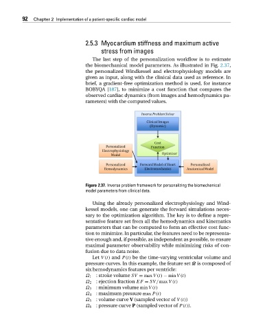
the biomechanical model parameters. As illustrated in Fig. 2.37,
the personalized Windkessel and electrophysiology models are
given as input, along with the clinical data used as reference. In
brief, a gradient-free optimization method is used, for instance
BOBYQA [187], to minimize a cost function that compares the
observed cardiac dynamics (from images and hemodynamics pa-
rameters) with the computed values.

Figure 2.37. Inverse problem framework for personalizing the biomechanical
model parameters from clinical data.

Using the already personalized electrophysiology and Wind-
kessel models, one can generate the forward simulations neces-
sary to the optimization algorithm. The key is to define a repre-
sentative feature set from all the hemodynamics and kinematics
parameters that can be computed to form an effective cost func-
tion to minimize. In particular, the features need to be representa-
tive enough and, if possible, as independent as possible, to ensure
maximal parameter observability while minimizing risks of con-
fusion due to data noise.
Let V(t) and P(t) be the time-varying ventricular volume and
pressure curves. In this example, the feature set Ω is composed of
six hemodynamics features per ventricle:
Ω 1 : stroke volume SV = maxV(t) − minV(t)
Ω 2 : ejection fraction EF = SV/maxV(t)
Ω 3 : minimum volume minV(t)
Ω 4 : maximum pressure maxP(t)
Ω 5 : volume curve V (sampled vector of V(t))
Ω 6 : pressure curve P (sampled vector of P(t)).