Page 110 - Artificial Intelligence for Computational Modeling of the Heart

80 Chapter 2 Implementation of a patient-specific cardiac model

as the collision operator and accounts for the contribution of the
collision between particles. For the numerical implementation of
LBM, Eq. (2.31) is written in a discrete form:

∂f i
+ c i ·∇f = K(f i ), (2.32)
∂t
where f i = f i (x,t) is a discrete representation of f with respect to
the variable u, more specifically instead of a single function f that
depends on u, x,and t, there are a finite number of f i functions
that depend on just x and t. The discrete velocities c i are associ-
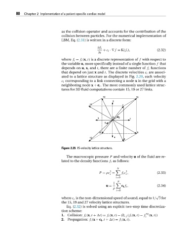
ated to a lattice structure as displayed in Fig. 2.29,eachvelocity
c i corresponding to a link connecting a node x in the grid with a
neighboring node x + e i . The most commonly used lattice struc-
tures for 3D fluid computations contain 15, 19 or 27 links.

Figure 2.29. 15-velocity lattice structure.

The macroscopic pressure P and velocity u of the fluid are re-
lated to the density functions f i as follows:

N
2 # 2
P = ρc = f i c , (2.33)
s s
i=0
N
1 #
u = c i f i , (2.34)
ρ
i=0
√
where c s is the non-dimensional speed of sound, equal to 1/ 3 for
the 15, 19 and 27 velocity lattice structures.
Eq. (2.32) is solved using an explicit two-step time discretiza-
tion scheme:
eq
1. Collision: f i (x,t + t) = f i (x,t) − Ω i,j (f i (x,t) − f (x,t))
i
2. Propagation: f i (x + c i ,t + t) = f i (x,t).