Page 107 - Artificial Intelligence for Computational Modeling of the Heart

Chapter 2 Implementation of a patient-specific cardiac model 77

Figure 2.26. A linear elastic beam of length l and height h is subject to a suddenly
applied shear stress S at one end while the other end is fixed.

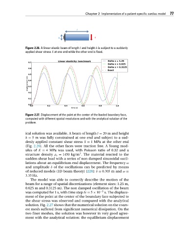
Figure 2.27. Displacement of the point at the center of the loaded boundary face,
computed with different spatial resolutions and with the analytical solution of the
problem.

ical solution was available. A beam of length l = 20 m and height
h = 5 m was fully constrained at one end and subject to a sud-
denly applied constant shear stress S = 1 MPa at the other end
(Fig. 2.26). All the other faces were traction free. A Young mod-
ulus of E = 4 MPa was used, with Poisson ratio of 0.32 and a
3
structure density ρ s = 1450 kg/m . The material reacted to the
sudden shear load with a series of non damped sinusoidal oscil-
lations about an equilibrium end displacement. The frequency ω
and amplitude δ of the oscillations can be predicted by means
of reduced models (1D beam theory) [228]: δ = 0.305 mand ω =
3.35 Hz.
The model was able to correctly describe the motion of the
beam for a range of spatial discretizations (element sizes: 1.25 m,
0.625 m and 0.3125 m). The non damped oscillation of the beam
was computed for 1 s, with time step δt = 5 × 10 −5 s. The displace-
ment of the point at the center of the boundary face subjected to
the shear stress was observed and compared with the analytical
solution. Fig. 2.27 shows that the numerical solution on the coars-
est mesh suffered from significant numerical dissipation. On the
two finer meshes, the solution was however in very good agree-
ment with the analytical solution: the equilibrium displacement