Page 104 - Artificial Intelligence for Computational Modeling of the Heart

74 Chapter 2 Implementation of a patient-specific cardiac model

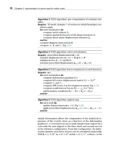
Algorithm 3 TLED algorithm: pre-computation of constant vari-
ables.
Require: 3D mesh, domain Γ of vertices to which boundary con-
ditions apply
for each tetrahedron do
compute initial volume V 0
compute spatial derivatives of the shape functions δh
compute linear strain-displacement matrices Z 0
end for
compute diagonal mass matrix M
compute A i , B i and C i (Eq. 2.27)

Algorithm 4 TLED algorithm: solver initialization.
Require: prescribed displacement d i∈Γ (0)
initialize displacements: u(−δt) ← 0, u(0) ← 0
initialize forces: f i (−δt) and f i (0)
initialize prescribed displacement u i∈Γ (0) ← d i∈Γ (0)

Algorithm 5 TLED algorithm: force computation at each iteration.
Require: u(t)
for each tetrahedron do
compute deformation gradient F(t)
compute full strain-displacement matrix Z(t) ← Z 0 F T
compute T a and T p
compute SPK tensor S at the integration points (Eq. 2.17)
T

compute nodal internal forces: f(t) ← Z(t) SdV 0
V 0
add boundary conditions f(t) ← f(t) + f bp (t) + f b (t)
end for
Algorithm 6 TLED algorithm: update step.
for each node do
update displacements u(u + δt) (Eq. 2.25)
apply prescribed displacements: u i∈Γ (t + δt) ← d i∈Γ (t + δt)
end for

simple deformation allows the computation of the analytical ex-
pression of the Cauchy stress as a function of the deformation
gradient F. A convenient set up to study simple shear is given by a
cube with the axes aligned to the fiber, sheet and normal vectors
in the reference configuration. From this configuration, the defor-
mation gradient and stress tensors can be calculated analytically.
T
T
T
With f 0 =[1,0,0] , s 0 =[0,1,0] and n 0 =[0,0,1] ,ashear γ in the