Page 128 - Artificial Intelligence for Computational Modeling of the Heart

100 Chapter 3 Learning cardiac anatomy

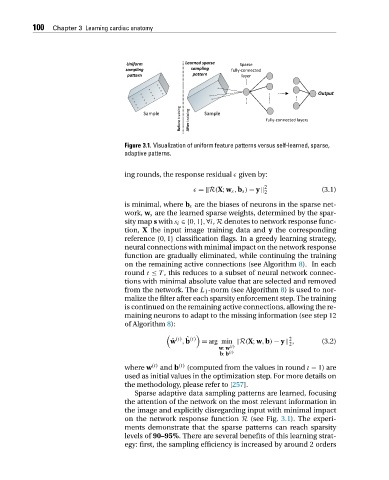
Figure 3.1. Visualization of uniform feature patterns versus self-learned, sparse,
adaptive patterns.

ing rounds, the response residual given by:
2
= R(X;w s ,b s ) − y 2 (3.1)
is minimal, where b s are the biases of neurons in the sparse net-
work, w s are the learned sparse weights, determined by the spar-
sity map s with s i ∈{0,1},∀i, R denotes to network response func-
tion, X the input image training data and y the corresponding
reference {0,1} classification flags. In a greedy learning strategy,
neural connections with minimal impact on the network response
function are gradually eliminated, while continuing the training
on the remaining active connections (see Algorithm 8). In each
round t ≤ T , this reduces to a subset of neural network connec-
tions with minimal absolute value that are selected and removed
from the network. The L 1 -norm (see Algorithm 8) is used to nor-
malize the filter after each sparsity enforcement step. The training
is continued on the remaining active connections, allowing the re-
maining neurons to adapt to the missing information (see step 12
of Algorithm 8):

(t) ˆ (t) 2
ˆ w ,b = arg min R(X;w,b) − y , (3.2)
2
w: w (t)
b: b (t)
where w (t) and b (t) (computed from the values in round t − 1)are
used as initial values in the optimization step. For more details on
the methodology, please refer to [257].
Sparse adaptive data sampling patterns are learned, focusing
the attention of the network on the most relevant information in
the image and explicitly disregarding input with minimal impact
on the network response function R (see Fig. 3.1). The experi-
ments demonstrate that the sparse patterns can reach sparsity
levels of 90–95%. There are several benefits of this learning strat-
egy: first, the sampling efficiency is increased by around 2 orders