Page 129 - Artificial Intelligence for Computational Modeling of the Heart

Chapter 3 Learning cardiac anatomy 101

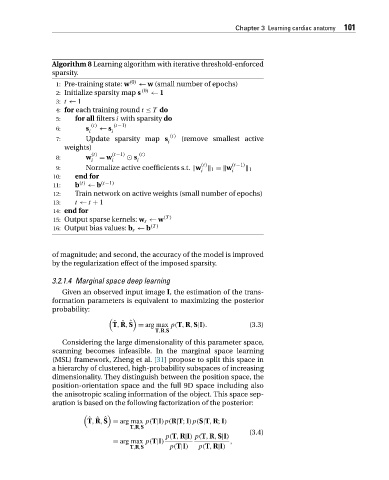
Algorithm 8 Learning algorithm with iterative threshold-enforced
sparsity.
1: Pre-training state: w (0) ← w (small number of epochs)
2: Initialize sparsity map s (0) ← 1
3: t ← 1
4: for each training round t ≤ T do
5: for all filters i with sparsity do
(t) (t−1)
6: s ← s
i i
7: Update sparsity map s (t) (remove smallest active
i
weights)
(t) (t−1) (t)
8: w = w s
i i i
(t)
9: Normalize active coefficients s.t. w 1 = w (t−1) 1
i i
10: end for
11: b (t) ← b (t−1)
12: Train network on active weights (small number of epochs)
13: t ← t + 1
14: end for
15: Output sparse kernels: w s ← w (T )
16: Output bias values: b s ← b (T )

of magnitude; and second, the accuracy of the model is improved
by the regularization effect of the imposed sparsity.

3.2.1.4 Marginal space deep learning
Givenanobservedinput image I, the estimation of the trans-
formation parameters is equivalent to maximizing the posterior
probability:

ˆ ˆ ˆ
T,R,S = arg max p(T,R,S|I). (3.3)
T,R,S
Considering the large dimensionality of this parameter space,
scanning becomes infeasible. In the marginal space learning
(MSL) framework, Zheng et al. [31] propose to split this space in
a hierarchy of clustered, high-probability subspaces of increasing
dimensionality. They distinguish between the position space, the
position-orientation space and the full 9D space including also
the anisotropic scaling information of the object. This space sep-
aration is based on the following factorization of the posterior:

ˆ ˆ ˆ
T,R,S = arg max p(T|I)p(R|T;I)p(S|T,R;I)
T,R,S
(3.4)
p(T,R|I) p(T,R,S|I)
= arg max p(T|I) ,
T,R,S p(T|I) p(T,R|I)