Page 183 - Artificial Intelligence for Computational Modeling of the Heart

Chapter 4 Data-driven reduction of cardiac models 155

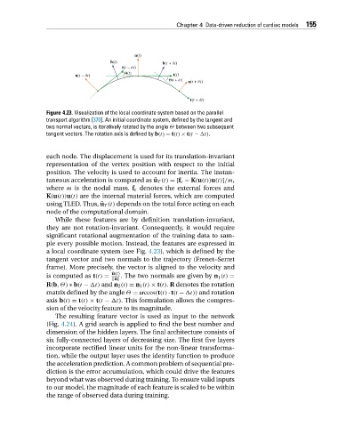
Figure 4.23. Visualization of the local coordinate system based on the parallel
transport algorithm [370]. An initial coordinate system, defined by the tangent and
two normal vectors, is iteratively rotated by the angle Θ between two subsequent
tangent vectors. The rotation axis is defined by b(t) = t(t) × t(t − t).

each node. The displacement is used for its translation-invariant
representation of the vertex position with respect to the initial
position. The velocity is used to account for inertia. The instan-
taneous acceleration is computed as ¨ u T (t) =[f e − K(u(t))u(t)]/m,
where m is the nodal mass. f e denotes the external forces and
K(u(t))u(t) are the internal material forces, which are computed
using TLED. Thus, ¨ u T (t) depends on the total force acting on each
node of the computational domain.
While these features are by definition translation-invariant,
they are not rotation-invariant. Consequently, it would require
significant rotational augmentation of the training data to sam-
ple every possible motion. Instead, the features are expressed in
a local coordinate system (see Fig. 4.23), which is defined by the
tangent vector and two normals to the trajectory (Frenet–Serret
frame). More precisely, the vector is aligned to the velocity and
˙ u(t)
is computed as t(t) = . The two normals are given by n 1 (t) =
˙ u
R(b,Θ) ∗ b(t − t) and n 2 (t) = n 1 (t) × t(t). R denotes the rotation
matrix defined by the angle Θ = arccos(t(t) · t(t − t)) and rotation
axis b(t) = t(t) × t(t − t). This formulation allows the compres-
sion of the velocity feature to its magnitude.
The resulting feature vector is used as input to the network
(Fig. 4.24). A grid search is applied to find the best number and
dimension of the hidden layers. The final architecture consists of
six fully-connected layers of decreasing size. The first five layers
incorporate rectified linear units for the non-linear transforma-
tion, while the output layer uses the identity function to produce
the acceleration prediction. A common problem of sequential pre-
diction is the error accumulation, which could drive the features
beyond what was observed during training. To ensure valid inputs
to our model, the magnitude of each feature is scaled to be within
the range of observed data during training.