Page 180 - Artificial Intelligence for Computational Modeling of the Heart

152 Chapter 4 Data-driven reduction of cardiac models

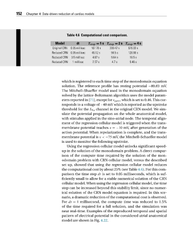
Table 4.6 Computational cost comparison.

Model dt T stop = 1s T stop = 2s T stop = 4s
Original CRN 0.05 millisec 167.78 s 339.42 s 676.03 s
Reduced CRN 0.05 millisec 46.12 s 94.5 s 128.88 s
Reduced CRN 0.5 millisec 4.67 s 9.64 s 18.5 s
Reduced CRN 1 millisec 2.57 s 4.7 s 9.46 s

which is registered to each time step of the monodomain equation
solution. The reference profile has resting potential −80.83 mV.
The Mitchell–Shaeffer model used in the monodomain equation
solved by the lattice-Boltzmann algorithm uses the model param-
eters reported in [71], except for v gate , which is set to 0.46. This cor-
responds to a voltage of −40 mV which is reported as the upstroke
threshold for the I Na channel in the original CRN model. We sim-
ulate the potential propagation on the whole anatomical model,
with stimulus applied in the sino-atrial node. The temporal align-
ment of the regression cellular model is triggered when the trans-
membrane potential reaches v =−10 mV, after generation of the
action potential. When repolarization is complete, and the trans-
membrane potential is v< −75 mV, the Mitchell–Schaeffer model
is used to monitor the following upstroke.
Using the regression cellular model unlocks significant speed-
up in the solution of the monodomain problem. A direct compar-
ison of the compute time required by the solution of the mon-
odomain problem with CRN cellular model, versus the described
set up, showed that using the regression cellular model reduces
the computational cost by about 25% (see Table 4.6). For this com-
parison thetimestep dt is set to 0.05 milliseconds, which is suf-
ficiently small to allow for a stable numerical solution of the CRN
cellular model. When using the regression cellular model, the time
step can be increased beyond this stability limit, since no numer-
ical solution of the CRN model equation is required. In this sce-
nario, a dramatic reduction of the computational cost is observed.
For dt = 1 millisecond, the compute time was reduced to 1.5%
of the time required for a full solution, and the simulation was
near real-time. Examples of the reproduced temporal and spatial
pattern of electrical potential in the considered atrial anatomical
model are shown in Fig. 4.22.