Page 48 - Artificial Intelligence for Computational Modeling of the Heart

18 Chapter 1 Multi-scale models of the heart for patient-specific simulations

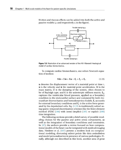
friction and viscous effects can be added into both the active and
passive models (μ and respectively η in the figure).

Figure 1.8. Illustration of an advanced version of the Hill–Maxwell rheological
model of cardiac biomechanics.

To compute cardiac biomechanics, one solves Newton’s equa-
tion of motion:

M ¨ u + D ˙ u + Ku = f a + f p + f b , (1.13)

u denotes the displacement vector of a material point at time t,
˙ u is the velocity and ¨ u the material point acceleration. M is the
mass matrix, D is the damping of the system, often chosen to
be of Rayleigh type, and K is the anisotropic stiffness matrix. f bp
captures the ventricular blood pressure, applied as a boundary
condition to the endocardial surface and computed by both my-
ocardium biomechanics and hemodynamics models. f b accounts
for external boundary conditions and f a is the active force gener-
ated by the depolarized cells. Eq. (1.13) is traditionally solved us-
ing spatio-temporal discretization schemes like the finite element
method (FEM) [104] with (semi-)implicit [105]orexplicit[106]
time integration.
The following sections provide a brief survey of possible mod-
eling choices for the passive and active stress components, as
well as the integration of boundary conditions and constraints.
In [47], the authors provide a review focused on how computa-
tional models of the heart can be integrated with medical imaging
data. Niederer et al. [107] present a modern look on computa-
tional modeling, discussing salient points like data assimilation
and model personalization in presence of various pathologies. Fi-
nally, although not described in this book, another area of great