Page 50 - Artificial Intelligence for Computational Modeling of the Heart

20 Chapter 1 Multi-scale models of the heart for patient-specific simulations

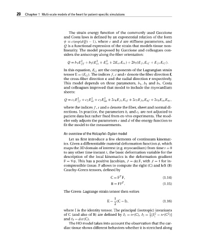
The strain energy function of the commonly used Guccione
and Costa laws is defined by an exponential relation of the form
ψ = c(exp(dQ) − 1),where c and d are stiffness parameters, and
Q is a functional expression of the strain that models tissue non-
linearity. The model proposed by Guccione and colleagues con-
siders the anisotropy along the fiber orientation:
2
2
Q = b 1 E 2 ff + b 2 (E + E + 2E cr E rc ) + 2b 3 (E fc E cf + E fr E rf ).
cc
rr
In this equation, E ij are the components of the Lagrangian strain
tensor E = (E ij ). The indices f , c and r denote the fiber direction f,
the cross-fiber direction c and the radial direction r respectively.
This model depends on three parameters, b 1 , b 2 and b 3 . Costa
and colleagues improved that model to include the myocardium
sheets:
2
2
Q = c 1 E ff + c 2 E + c 3 E 2 nn + 2c 4 E fs E sf + 2c 5 E fn E nf + 2c 6 E sn E ns ,
ss
where the indices f , s and n denote the fiber, sheet and normal di-
rections. In practice, the parameters b i and c i are not adjusted to
patient data but rather fixed from ex-vivo experiments. The mod-
eler only adjusts the parameters c and d of the energy function to
fit the model to the measurements.

An overview of the Holzapfel–Ogden model
Let us first introduce a few elements of continuum kinemat-
ics. Given a differentiable material deformation function φ,which
maps the 3D domain of interest (e.g. myocardium) from time t = 0
to any other time instant t, the basic deformation variable for the
description of the local kinematics is the deformation gradient
F =∇φ. This has a positive Jacobian, J = detF, with J = 1 for in-
compressible tissue. F allows to compute the right (C) and left (B)
Cauchy–Green tensors, defined by
T
C = F F, (1.14)
T
B = FF . (1.15)
The Green–Lagrange strain tensor then writes

1
E = (C − I), (1.16)
2
where I is the identity tensor. The principal (isotropic) invariants
1 2 2
of C (and also of B) are defined by I 1 = tr(C), I 2 = [I − tr(C )]
2 1
and I 3 = det(C).
The HO model takes into account the observation that the car-
diac tissue shows different behaviors whether it is stretched along