Page 43 - Artificial Intelligence for Computational Modeling of the Heart

Chapter 1 Multi-scale models of the heart for patient-specific simulations 13

ation and propagation, this approach significantly simplifies the
mathematical formulation as a traveling wave problem, expressed
using an anisotropic Eikonal equation [77–79]. Such models are
governed by very few parameters and they can be solved very effi-
ciently using anisotropic fast marching methods [80,81]orgraph-
based techniques [82]. They are therefore suited for real-time sim-
ulations as one full-heart depolarization can be simulated in sec-
onds. Relatively recently, advanced implementation techniques
enabled to simulate wave reentry [83], which was believed to be
out of reach for such models. However, because of the extreme
simplifications introduced in the model, pathological phenomena
like arrhythmias, fibrillations or tachycardia cannot be simulated.

One example: a monodomain model
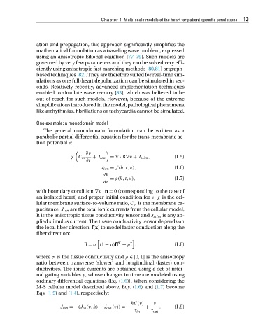
The general monodomain formulation can be written as a
parabolic partial differential equation for the trans-membrane ac-
tion potential v:
∂v

χ C m + J ion =∇ · R∇v + J stim , (1.5)
∂t
J ion = f(h,t,v), (1.6)
dh
= g(h,t,v), (1.7)
dt
with boundary condition ∇v · n = 0 (corresponding to the case of
an isolated heart) and proper initial condition for v. χ is the cel-
lular membrane surface-to-volume ratio, C m is the membrane ca-
pacitance, J ion are the total ionic currents from the cellular model,
R is the anisotropic tissue conductivity tensor and J stim is any ap-
plied stimulus current. The tissue conductivity tensor depends on
the local fiber direction, f(x) to model faster conduction along the
fiber direction:

T
R = σ (1 − ρ)ff + ρI , (1.8)
where σ is the tissue conductivity and ρ ∈[0,1] is the anisotropy
ratio between transverse (slower) and longitudinal (faster) con-
ductivities. The ionic currents are obtained using a set of inter-
nal gating variables y, whose changes in time are modeled using
ordinary differential equations (Eq. (1.6)). When considering the
M-S cellular model described above, Eqs. (1.6)and(1.7)become
Eqs. (1.9)and (1.4), respectively:

hC(v) v
J ion =−(J in (v,h) + J out (v)) =− + . (1.9)
τ in τ out