Page 93 - Artificial Intelligence for Computational Modeling of the Heart

Chapter 2 Implementation of a patient-specific cardiac model 63

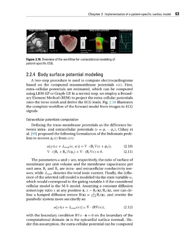
Figure 2.18. Overview of the workflow for computational modeling of
patient-specific ECG.

2.2.4 Body surface potential modeling
A two-step procedure is used to compute electrocardiograms
based on the computed transmembrane potentials v(t).First,
extra-cellular potentials are estimated, which can be computed
using LBM-EP or Graph-EP. In a second step, we employ a Bound-
ary Element Method (BEM) to project the extra-cellular potentials
onto the torso mesh and derive the ECG leads. Fig. 2.18 illustrates
the complete workflow of the forward model from images to ECG
signals.

Extracellular potentials computation
Defining the trans-membrane potentials as the difference be-
tween intra- and extracellular potentials (v = φ i − φ e ), Chhay et
al. [99] proposed the following formulation of the bidomain prob-
lem to recover φ e (t) from v(t):

α[γ∂ t v + J total (v,w)]=∇ · (R i ∇(v + φ e )), (2.10)
∇· ((R i + R e )∇φ e ) +∇ · (R i ∇v) = 0. (2.11)
The parameters α and γ are, respectively, the ratio of surface of
membrane per unit volume and the membrane capacitance per
unit area. R i and R e are intra- and extracellular conductivity ten-
sors, while J total denotes the total ionic current. Finally, the influ-
ence of the selected cell model is modeled via the state variable w,
which would correspond to the gating variable h if the considered
cellular model is the M-S model. Assuming a constant diffusion
anisotropy ratio λ at any position x, λ = R i (x)/R e (x),one cande-
1
fine a lumped diffusion tensor R(x) = R i (x), and rewrite the
1+λ
parabolic system more succinctly as:
α[γ∂ t v + J total (v)]=∇ · (R∇(v)), (2.12)
with the boundary condition R∇v · n = 0 on the boundary of the
computational domain (n is the epicardial surface normal). Un-
der this assumption, the extra-cellular potential can be computed