Page 97 - Artificial Intelligence for Computational Modeling of the Heart

Chapter 2 Implementation of a patient-specific cardiac model 67

with u the vector of nodal displacements, f a theactiveforceof
the depolarized cells, f bp the endocardial pressure, f b the exter-
nal forces and K(u) the stiffness matrix, non-linearly dependent
on the deformation. D represents a Rayleigh-type damping, i.e.
D = λ M M + λ K K, with λ M and λ K user-defined scalar coefficients.
The dynamics equaton (2.15) is traditionally solved by using
the finite element method (FEM) with a hexahedral or tetrahedral
spatial discretization of the myocardial domain, although finite
difference [130] and mesh-less [224,225] approaches have also
been explored. Using the FEM, the equation is solved on the mesh
nodes, with the nodal forces calculated by accumulating the con-
tributions of all elements sharing common nodes. A particularly
efficient algorithm, using the FEM and explicit central difference
temporal discretization of Eq. (2.15)(seee.g.[104], p. 803), is the
Total Lagrangian Explicit Dynamics (TLED) algorithm, originally
proposed by Miller et al. [106]. Its main idea is to refer all math-
ematical quantities of interest to the original undeformed config-
uration of the system. Such a formulation allows to pre-compute
several quantities, thus reducing the amount of mathematical op-
erations to be done at each time step. Furthermore, TLED uses low
order polynomial approximation for the unknowns of the equa-
tion and a lumped mass approximation [104] (such that M is a di-
agonal matrix). This, combined with the explicit time integration
scheme, results in computationally inexpensive time stepping. At
each time step no matrix inversion is required (as would be the
case for implicit or semi-implicit time advancing algorithms) and
operations are node-wise, hence massively parallelizable on GPU
for instance. For these reasons, TLED is particularly suitable for
real-time computation of soft tissue deformations like brain, liver,
kidney [106]. Mathematical formulations for the cardiac use case
are provided below, following the approach presented in [226].
Let φ be the differentiable material deformation function, F =
∇φ the deformation gradient, J = detF the Jacobian determinant,
T
and C = F F the right Cauchy–Green tensor. Myocardium biome-
chanics is modeled using a Hill–Maxwell framework (section 1.3),
which decomposes the total Cauchy stress T into the sum of its
active and passive parts, T = T a − T p . The negative sign associ-
ated to the passive stress appears as the stiffness matrix K(u) is in
the left-hand side of Eq. (2.15), whereas the active stress is in the
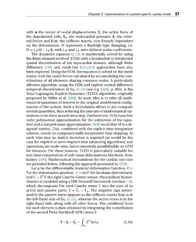
right-hand side, along with all other forces. The combined force
for each element is then obtained by integrating the contribution
of the second Piola-Kirchhoff (SPK) stress S

T
f = f a − f p = Z SdV 0 (2.16)
V 0