Page 92 - Artificial Intelligence for Computational Modeling of the Heart

62 Chapter 2 Implementation of a patient-specific cardiac model

ocardium and R is a symmetric conductivity tensor:

T
R = σ 2 (1 − ρ)ff + ρI (2.8)
σ is the local conduction velocity (along the fiber direction), ρ ∈
[0,1] is the anisotropy ratio, I the identity matrix and f the fiber
direction.
A very efficient numerical solution of the Eikonal equation is
based on a variant of Dijkstra’s shortest path algorithm [82]. The
input of the method is the tetrahedral mesh of the patient’s heart,
which is tagged to identify where the EP wave starts (left and right
ventricular septum, see also Fig. 2.16). As a first step, the nodes
from where the electrical wave starts are added to a priority queue,
with a value equal to their activation time. For instance, the LV
septum nodes are added with their prescribed activation time a LV ,
and the RV septum nodes with their prescribed activation time
a RV . Any additional activation point (e.g. due to device pacing)
can be added to the priority queue based on its own activation
time. The first node of the queue is then selected and all its neigh-
bors are processed.
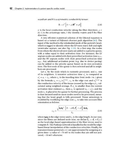
Let n i be the node which is currently processed, and n j one
of its neighbors. A tentative activation time a is computed as

j

a = a i + t ij ,where t ij is the traveling time from node i to j given
j
by the formula t ij = c ij /σ tissue , c ij istheedgecostand σ tissue is
ij ij
the conduction velocity of the tissue crossed by the edge n i n j , cal-

culated using weighted average. If a is smaller than the current
j

activation time estimate a j ,then a j is updated (a j = a ), and the
j
node n j is placed in the queue for further processing. The process
is then iterated until no more nodes need to be processed, mean-
ing that the heart graph is fully processed. Tissue anisotropy is
modeled by modifying the edge cost c ij to take into account fiber
orientation as follows:

T T
n i n j (1 − ρ)f ij f + ρI n i n j
ij
c ij = (2.9)
δ ij
where n i n j is the edge vector and δ ij is theedgelength.Inourcase,
since the fibers are defined node wise, we define f ij = (f i + f j )/2
as the local edge-based approximation of the fiber vector, used to
compute R. The Purkinje network is handled in the model by edge-
based linear interpolation of the conduction velocities. Finally, the
transmembrane potentials v(t) are approximated by assigning at a
given time t avalueof −70 mV to the nodes that are still not acti-
vated, +30 mV otherwise.