Page 443 - Automotive Engineering Powertrain Chassis System and Vehicle Body

CHAP TER 1 4. 2 Decisional architecture

kinematic and dynamic constraints of the vehicle. In a
previous approach, a fuzzy controller combining different
basic behaviours (trajectory tracking, obstacle avoidance,
etc.) was used to perform trajectory following (Garnier
and Fraichard, 1996). However this approach proved
unsatisfactory: it yields oscillating behaviours, and does
not guarantee that all the aforementioned constraints are
always satisfied.
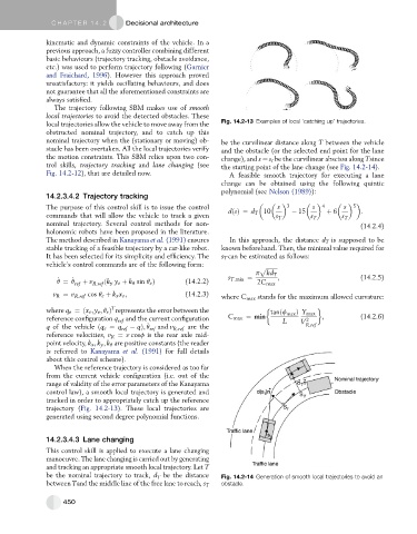
The trajectory following SBM makes use of smooth
local trajectories to avoid the detected obstacles. These
local trajectories allow the vehicle to move away from the Fig. 14.2-13 Examples of local ‘catching up’ trajectories.
obstructed nominal trajectory, and to catch up this
nominal trajectory when the (stationary or moving) ob- be the curvilinear distance along T between the vehicle
stacle has been overtaken. All the local trajectories verify and the obstacle (or the selected end point for the lane
the motion constraints. This SBM relies upon two con- change), and s ¼ s t be the curvilinear abscissa along Tsince
trol skills, trajectory tracking and lane changing (see the starting point of the lane change (see Fig. 14.2-14).
Fig. 14.2-12), that are detailed now. A feasible smooth trajectory for executing a lane
change can be obtained using the following quintic
polynomial (see Nelson (1989)):
14.2.3.4.2 Trajectory tracking

The purpose of this control skill is to issue the control dðsÞ¼ d T 10 s 3 15 s 4 þ 6 s 5
commands that will allow the vehicle to track a given s T s T s T :
nominal trajectory. Several control methods for non- (14.2.4)
holonomic robots have been proposed in the literature.
The method described in Kanayama et al. (1991) ensures In this approach, the distance d T is supposed to be
stable tracking of a feasible trajectory by a car-like robot. known beforehand. Then, the minimal value required for
It has been selected for its simplicity and efficiency. The s T can be estimated as follows:
vehicle’s control commands are of the following form: p ffiffiffiffiffiffiffiffi
p kd T
s T:min ¼ ; (14.2.5)
_
q ¼ q _ ref þ v R:ref ðk y y e þ k q sin q e Þ (14.2.2) 2C max
v R ¼ v R:ref cos q e þ k x x e ; (14.2.3) where C max stands for the maximum allowed curvature:
T
where q e ¼ðx e ; y e ; q e Þ represents the error between the tanðf max Þ Y max
reference configuration q ref and the current configuration C max ¼ min L V 2 ; (14.2.6)
q of the vehicle ðq e ¼ q ref qÞ; q _ ref and v R:ref are the R:ref
reference velocities, v R ¼ v cosf is the rear axle mid-
point velocity, k x ; k y ; k q are positive constants (the reader
is referred to Kanayama et al. (1991) for full details
about this control scheme).
When the reference trajectory is considered as too far
from the current vehicle configuration (i.e. out of the
range of validity of the error parameters of the Kanayama
control law), a smooth local trajectory is generated and
tracked in order to appropriately catch up the reference
trajectory (Fig. 14.2-13). These local trajectories are
generated using second degree polynomial functions.

14.2.3.4.3 Lane changing
This control skill is applied to execute a lane changing
manoeuvre. The lane changing is carried out by generating
and tracking an appropriate smooth local trajectory. Let T
be the nominal trajectory to track, d T be the distance Fig. 14.2-14 Generation of smooth local trajectories to avoid an
between Tand the middle line of the free lane to reach, s T obstacle.

450